
What is the taxi cab theory? It’s a journey into a world where straight lines bend to the rigid geometry of city streets, a realm where distance isn’t as the crow flies, but as the cabbie drives. Prepare to unravel the mysteries of Manhattan distance, a concept that transcends mere mathematics, reaching into the very fabric of urban planning, robotics, and even the digital landscapes of image processing.
This is not merely a theoretical exercise; it’s a practical exploration of how we measure space, how we navigate it, and how we understand the world around us.
Imagine a city grid, a labyrinth of avenues and streets, each a constraint on the freedom of movement. This is the canvas upon which the taxi cab theory unfolds. Forget the elegant curves of Euclidean geometry; here, we deal with the sharp angles, the abrupt turns, the relentless march of blocks. We’ll delve into the mathematical underpinnings of this unique geometric system, examining the formula for calculating distances, the peculiar shapes of “circles,” and the unexpected properties of lines.
Through examples and visualizations, we’ll witness the power and limitations of this unconventional approach to spatial measurement.
Introduction to the Taxi Cab Geometry

Taxi cab geometry, also known as Manhattan geometry, is a fascinating alternative to the familiar Euclidean geometry we learn in school. It’s a non-Euclidean geometry where the distance between two points is measured along a grid, mimicking the way a taxi might travel in a city with a rectangular grid of streets. Instead of the straight-line distance, we consider the sum of the horizontal and vertical distances.Taxi cab geometry fundamentally alters our understanding of distance.
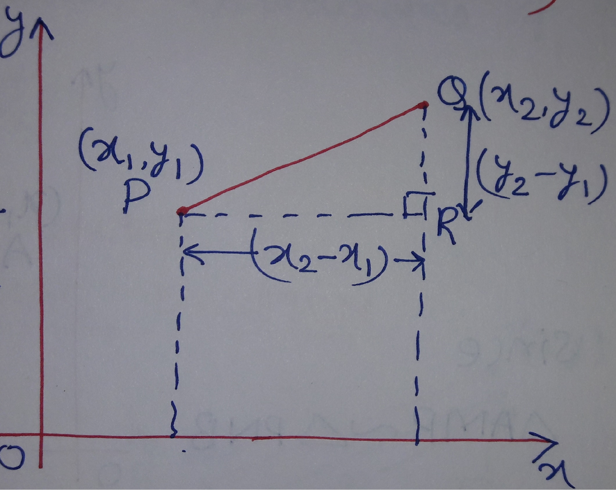
While Euclidean geometry uses the Pythagorean theorem to calculate distance (√((x₂-x₁)² + (y₂-y₁)²) ), taxi cab geometry simply adds the absolute differences in the x and y coordinates: |x₂
- x₁| + |y₂
- y₁|. This seemingly simple change leads to a rich and surprisingly different geometric landscape.
Euclidean versus Taxi Cab Distances
The core difference between Euclidean and taxi cab distances lies in how they account for obstacles and restrictions on movement. Euclidean distance represents the shortest distance between two points
as the crow flies*, ignoring any physical barriers. Taxi cab distance, on the other hand, reflects a more realistic scenario, especially in urban environments, where movement is constrained to a grid. Imagine two points on a map
in Euclidean geometry, the shortest path is a straight line. In taxi cab geometry, the shortest path is along the grid lines, creating a path that is often longer than the Euclidean distance. For example, consider two points (0,0) and (3,4). The Euclidean distance is √(3² + 4²) = 5. The taxi cab distance is |3-0| + |4-0| = 7.
This difference highlights the practical limitations imposed by the grid structure.
Real-World Applications of Taxi Cab Geometry
Taxi cab geometry finds practical applications in various fields beyond simply calculating taxi fares. One significant area is urban planning and transportation. Optimizing routes for delivery services, emergency vehicles, or public transportation often involves minimizing travel time along a grid-like street network, making taxi cab geometry a valuable tool for route optimization algorithms. Furthermore, network analysis, particularly in computer science, utilizes taxi cab geometry to model connections and distances in networks where connections are limited to specific paths or nodes.
Image analysis and robotics also benefit from this geometry, particularly in scenarios involving movement on a grid or in environments with obstacles that restrict movement to specific directions. The efficiency of algorithms for pathfinding and navigation in such environments can be improved using taxi cab geometry principles.
Defining Taxi Cab Distance
Taxi cab distance, also known as Manhattan distance or L1 distance, offers a unique perspective on measuring the distance between points, differing significantly from the familiar Euclidean distance. Its name derives from the grid-like street layout of Manhattan, where travel distances are constrained by the city’s orthogonal structure. Understanding its mathematical definition, properties, and applications is crucial for appreciating its distinct role in various fields.
Mathematical Notation and Definition
Taxi cab distance between two points (x₁, y₁) and (x₂, y₂) in a 2D Cartesian coordinate system is defined as the sum of the absolute differences of their Cartesian coordinates. The formula is:
dtaxi((x₁, y₁), (x₂, y₂)) = |x₂
- x₁| + |y₂
- y₁|
This definition extends to n-dimensional spaces as:
dtaxi((x₁ 1, x₁ 2,…, x₁ n), (x₂ 1, x₂ 2,…, x₂ n)) = Σ i=1n |x₂ i
x₁i|
Let’s illustrate with examples:* Example 1: (2, 3) and (5, 7) d taxi((2, 3), (5, 7)) = |5 – 2| + |7 – 3| = 3 + 4 = 7* Example 2: (-1, 0) and (3, -2) d taxi((-1, 0), (3, -2)) = |3 – (-1)| + |-2 – 0| = 4 + 2 = 6* Example 3: (0, 0, 0) and (1, 2, 3) in 3D space d taxi((0, 0, 0), (1, 2, 3)) = |1 – 0| + |2 – 0| + |3 – 0| = 1 + 2 + 3 = 6
Properties of Taxi Cab Distance
Taxi cab distance satisfies the four properties of a metric:
- Non-negativity: d taxi(p, q) ≥ 0 for all points p and q. This is evident from the definition, as the sum of absolute values is always non-negative.
- Identity of indiscernibles: d taxi(p, q) = 0 if and only if p = q. The sum of absolute differences is zero only when all corresponding coordinates are identical.
- Symmetry: d taxi(p, q) = d taxi(q, p). The absolute difference |x₂
-x₁| is equal to |x₁
-x₂|, ensuring symmetry. - Triangle inequality: d taxi(p, r) ≤ d taxi(p, q) + d taxi(q, r) for all points p, q, and r. This can be proven by considering the individual coordinate differences and applying the triangle inequality for real numbers: |a + b| ≤ |a| + |b|.
Taxi cab distance differs from Euclidean distance (straight-line distance) in its geometric interpretation and resulting distance values. Euclidean distance is calculated using the Pythagorean theorem, resulting in a shorter distance compared to the taxi cab distance in most cases.
| Metric Name | Formula | Geometric Interpretation | Properties | Applications |
|---|---|---|---|---|
| Euclidean Distance | √((x₂
| Straight-line distance | Non-negativity, Identity of indiscernibles, Symmetry, Triangle inequality | Navigation, physics, image processing |
| Taxi Cab Distance | |x₂
| Distance along grid lines | Non-negativity, Identity of indiscernibles, Symmetry, Triangle inequality | Robotics, image analysis, data mining |
The non-Euclidean nature of taxi cab distance stems from its reliance on a grid structure, unlike the Euclidean distance’s consideration of the shortest path regardless of the underlying geometry. This affects applications where movement is restricted to a grid, such as city navigation or robot movement in a grid-based environment.
Calculation Methods and Algorithms
A basic iterative approach to calculating taxi cab distance directly implements the formula:“`function taxiCabDistance(point1, point2): distance = 0 for i from 0 to length(point1)
1
distance = distance + abs(point2[i]
point1[i])
return distance“`A vectorized approach, utilizing vector operations, can be more efficient for large datasets:“`function taxiCabDistanceVectorized(point1, point2): return sum(abs(point2 – point1))“`The time complexity of both algorithms is O(n), where n is the dimensionality of the space. Matrix operations can efficiently compute taxi cab distances between multiple points. For instance, if we have a matrix A representing a set of points, the pairwise taxi cab distances can be computed using matrix operations involving absolute differences and summation.Computational optimizations for high-dimensional spaces might include techniques like dimensionality reduction or approximate nearest neighbor search algorithms.
Applications and Visualization
Taxi cab distance finds applications in:
- City Navigation: Calculating travel time or distance in cities with grid-like street layouts.
- Robotics: Planning paths for robots moving on a grid.
- Image Processing: Measuring similarity between images based on pixel differences.
Imagine two points A (2,1) and B (5,4) on a grid. The Euclidean distance is the straight line connecting A and B. The taxi cab distance is represented by the path a taxi would take, moving along the grid lines: three units to the right, and three units up, for a total distance of six units. This visually illustrates the difference between the two metrics.
A diagram could show this clearly, with the straight-line Euclidean distance and the step-wise taxi cab path both clearly marked.
Advanced Considerations
Taxi cab geometry, based on taxi cab distance, possesses unique properties. For instance, circles are actually squares rotated 45 degrees. The relationship between taxi cab distance and other metrics, such as Chebyshev distance (maximum coordinate difference), is that Chebyshev distance represents the limiting case of taxi cab distance as the weight on the coordinate differences approaches infinity. In image processing, taxi cab distance is used for feature extraction and pattern recognition.
Data mining employs it in clustering algorithms where data points are represented in a high-dimensional space.
Taxi Cab Circles
Taxi cab geometry, a fascinating alternative to Euclidean geometry, offers a unique perspective on distance and shape. Instead of the familiar straight-line distance, taxi cab geometry utilizes the distance a taxi would travel along a grid of streets, hence the name. This leads to surprising and counter-intuitive results, especially when we examine the concept of a “circle.”
Shape and Characteristics of Taxi Cab Circles
A taxi cab circle, unlike its Euclidean counterpart, is not a smooth curve. It’s a polygon, formed by the set of all points equidistant from a central point, using the taxi cab metric. Consider a taxi cab circle with a radius of 5 units centered at the origin (0,0). Points on its perimeter will satisfy the equation |x| + |y| = 5.
Four points on the perimeter are (5,0), (0,5), (-5,0), and (0,-5). Other points include (4,1), (3,2), (2,3), (1,4), and their reflections across the axes. Increasing the radius to 10 units simply scales the shape; the perimeter points would be (10,0), (0,10), (-10,0), (0,-10), etc., resulting in a larger, similar polygon. The key difference lies in the definition of “distance.” In Euclidean geometry, distance is the straight-line length; in taxi cab geometry, distance is the sum of the absolute differences in x and y coordinates.
This difference fundamentally alters the shape of the circles. The mathematical equation for a taxi cab circle centered at (x c, y c) with radius r is |x – x c| + |y – y c| = r.
Comparison with Euclidean Circles
A Euclidean circle of radius r encloses an area of πr², while the area of a taxi cab circle of radius r is 2r². The perimeter of a Euclidean circle is 2πr, a smooth continuous curve. The perimeter of a taxi cab circle is more complex to calculate and depends on the radius, involving a summation of segments.
Consider a radius of 5 units:
| Characteristic | Euclidean Circle (r=5) | Taxi Cab Circle (r=5) |
|---|---|---|
| Radius | 5 | 5 |
| Area | 25π ≈ 78.54 | 50 |
| Perimeter/Circumference | 10π ≈ 31.42 | 20 |
| Shape Description | Smooth, continuous curve | Square-like polygon |
| Equation | (x-xc)² + (y-yc)² = r² | |x – xc| + |y – yc| = r |
The circumference of a taxi cab circle is significantly different from that of a Euclidean circle. While a precise formula for the perimeter is complex, approximations can be derived based on the radius and the number of sides of the resulting polygon.
Visual Representation of Taxi Cab Circles
A taxi cab circle with a radius of 7 units centered at (3,2) can be textually represented as follows (using “*” for perimeter points and ” ” for interior):“`
*
“`Creating a precise visual representation of a taxi cab circle is challenging because of its angular nature. Unlike the smooth curve of a Euclidean circle, the taxi cab circle is composed of straight line segments, creating a more blocky, less visually appealing representation. The visual appearance is best described as a rotated square, with corners that are more pronounced and less rounded than those of a Euclidean circle.
Its characteristic feature is its distinctly non-smooth, angular perimeter.
Advanced Considerations
Taxi cab geometry finds applications in urban planning, where the distance between two points is often measured along street grids. Network routing algorithms can also benefit from this geometry, optimizing routes based on the “taxi cab” distance. For example, determining the shortest route for a delivery service in a city with a grid-like street layout, or optimizing network traffic flow in a city with a structured road system.
Writing a Short Explanation of Taxi Cab Geometry
Taxi cab geometry is a way of measuring distance differently than we usually do. Instead of the “as the crow flies” straight-line distance of Euclidean geometry, taxi cab geometry measures distance as if you were driving a taxi along a grid of streets, only able to move horizontally or vertically. This means that the shortest distance between two points is not always a straight line.
A “circle” in taxi cab geometry isn’t round; it’s a square rotated at 45 degrees, representing all points equidistant from a center point using the taxi-cab distance. This seemingly simple change leads to fascinating differences in how we understand shapes and distances.
Taxi Cab Lines: What Is The Taxi Cab Theory
Unlike Euclidean geometry, where lines are defined by a constant slope and the equation y = mx + c, taxi cab geometry introduces a unique perspective on lines. Taxi cab lines, also known as taxicab lines, represent the shortest paths between two points when movement is restricted to horizontal and vertical directions, mimicking the movement of a taxi on a gridded city map.
This restriction significantly alters the properties of lines compared to their Euclidean counterparts.Taxi cab lines are characterized by their piecewise linear nature. They consist of segments parallel to the x-axis and the y-axis. The path of a taxi cab line is never diagonal. This means that the slope, in the traditional Euclidean sense, is not a consistent value along the entire line.
Instead, we encounter a more complex concept of taxi cab slope.
Taxi Cab Slopes
The concept of slope in taxi cab geometry differs fundamentally from its Euclidean counterpart. In Euclidean geometry, the slope is a single value representing the ratio of the vertical change to the horizontal change between any two points on the line. In contrast, taxi cab lines have multiple slopes: a horizontal slope of 0 and a vertical slope which is undefined.
A taxi cab line will have a slope of 0 for its horizontal segments and an undefined slope for its vertical segments. Consider two points A(2,3) and B(5,7). The Euclidean slope is (7-3)/(5-2) = 4/3. However, a taxi cab line connecting these points could involve moving horizontally from (2,3) to (5,3) and then vertically from (5,3) to (5,7), demonstrating the piecewise nature of the taxi cab line.
The slope along the horizontal segment is 0, and the slope along the vertical segment is undefined. This concept illustrates the difference between the two geometric systems.
Differences Between Taxi Cab Lines and Euclidean Lines
Several key distinctions exist between taxi cab lines and Euclidean lines. First, Euclidean lines are defined by a single, constant slope, whereas taxi cab lines are composed of segments with slopes of 0 (horizontal) and undefined (vertical). Second, Euclidean lines are continuous and infinitely extendable in both directions, while taxi cab lines consist of discrete, connected segments that maintain the restriction of horizontal and vertical movement.
A Euclidean line has only one path between two points, while there can be many paths connecting two points with a taxi cab line, although only one of these will represent the shortest distance. Finally, the concept of distance itself differs. In Euclidean geometry, distance is calculated using the Pythagorean theorem; in taxi cab geometry, it’s the sum of the absolute differences in x and y coordinates.
This difference fundamentally impacts how lines are defined and perceived within each geometry.
Taxi Cab Geometry in Different Dimensions
Taxi cab geometry, unlike Euclidean geometry, defines distance as the sum of the absolute differences between coordinates. This seemingly simple alteration leads to fascinating differences in higher dimensions, impacting our understanding of shapes and distances. Let’s explore how this unique metric extends beyond the familiar two and three dimensions.
Generalization of the Distance Formula and Implications for Circles and Spheres
The taxi cab distance formula generalizes readily to n dimensions. For two points, A and B, with coordinates (a₁, a₂, …, aₙ) and (b₁, b₂, …, bₙ) respectively, the taxi cab distance, denoted as d TC(A, B), is given by:
dTC(A, B) = |a₁
- b₁| + |a₂
- b₂| + … + |aₙ
- bₙ|
This formula directly extends the 2D and 3D cases. In Euclidean geometry, circles and spheres are smooth, continuous curves. However, in taxi cab geometry, these shapes become quite different. A taxi cab circle is a square rotated 45 degrees, while a taxi cab sphere in 3D is an octahedron. This is because the set of points equidistant from a central point under the taxi cab metric forms these shapes.
The “radius” in this context represents the sum of the absolute differences in coordinates, not the straight-line distance.
Examples of Calculations in 3D Taxi Cab Geometry
Here are three examples demonstrating taxi cab distance calculations in 3D: Example 1: Find the taxi cab distance between A(1, 2, 3) and B(4, 6, 9).d TC(A, B) = |1 – 4| + |2 – 6| + |3 – 9| = |-3| + |-4| + |-6| = 3 + 4 + 6 = 13 units Example 2: Find the taxi cab distance between A(0, 0, 0) and B(3, 4, 5).d TC(A, B) = |0 – 3| + |0 – 4| + |0 – 5| = |-3| + |-4| + |-5| = 3 + 4 + 5 = 12 units Example 3: Find the taxi cab distance between A(-2, 1, -1) and B(2, -3, 2).d TC(A, B) = |-2 – 2| + |1 – (-3)| + |-1 – 2| = |-4| + |4| + |-3| = 4 + 4 + 3 = 11 units
Taxi Cab and Euclidean Distances in 2D and 3D
The following table compares taxi cab and Euclidean distances for several point pairs:
| Point A | Point B | Taxi Cab Distance (units) | Euclidean Distance (units) |
|---|---|---|---|
| (1, 2) | (4, 6) | 7 | 5 |
| (0, 0) | (3, 4) | 7 | 5 |
| (-2, 1) | (2, -3) | 10 | 6.4 |
| (1, 2, 3) | (4, 6, 9) | 13 | √(9+16+36) = √61 ≈ 7.81 |
| (0, 0, 0) | (3, 4, 5) | 12 | √(9+16+25) = √50 ≈ 7.07 |
| (-2, 1, -1) | (2, -3, 2) | 11 | √(16+16+9) = √41 ≈ 6.4 |
Taxi Cab Circles in 2D and 3D
A 2D taxi cab circle with radius 4 centered at the origin is a square with vertices at (4,0), (0,4), (-4,0), (0,-4). The “radius” is the sum of the absolute differences in coordinates from the center. A 3D taxi cab circle with radius 6 is an octahedron with vertices at (6,0,0), (-6,0,0), (0,6,0), (0,-6,0), (0,0,6), (0,0,-6). The shape is determined by all points whose coordinate differences sum to 6.
Comparison of Taxi Cab and Euclidean Circles
Euclidean circles are smooth, continuous curves defined by points equidistant from a center. Taxi cab circles, however, are squares (in 2D) or octahedra (in 3D) with sharp corners. The concept of “radius” differs significantly. In Euclidean geometry, the radius is the straight-line distance; in taxi cab geometry, it’s the sum of absolute coordinate differences. This difference arises from the different distance metrics used.
Taxi Cab Spheres in Higher Dimensions
A taxi cab sphere in n-dimensional space is the set of all points whose taxi cab distance from a center point is a constant value, r. Mathematically, it can be represented as:
x ∈ ℝⁿ : Σᵢ₌₁ⁿ |xᵢ
cᵢ| = r
where x = (x₁, x₂, …, xₙ) is a point in n-dimensional space, c = (c₁, c₂, …, cₙ) is the center point, and r is the radius. The shape becomes increasingly complex as the number of dimensions increases.
Applications of Taxi Cab Geometry
Taxi cab geometry finds applications in scenarios where movement is restricted to a grid-like structure, mimicking city streets or network connections. Example 1: City planning and route optimization: Calculating shortest routes for delivery services or emergency vehicles in a city grid. The taxi cab distance directly reflects the actual distance traveled along city blocks. Example 2: Network analysis: Analyzing shortest paths in networks where connections are directional and movement is restricted to specific links.
Python Code for Taxi Cab Distance in n Dimensions
“`pythonimport numpy as npdef taxi_cab_distance(point_a, point_b): “””Calculates the taxi cab distance between two points in n-dimensional space. Args: point_a: A list or numpy array representing the coordinates of the first point. point_b: A list or numpy array representing the coordinates of the second point. Returns: The taxi cab distance between the two points.
“”” return np.sum(np.abs(np.array(point_a)
np.array(point_b)))
# Example usage:point_a = [1, 2, 3, 4]point_b = [5, 6, 7, 8]distance = taxi_cab_distance(point_a, point_b)print(f”The taxi cab distance between point_a and point_b is: distance”)“`
Applications of Taxi Cab Geometry
Taxi cab geometry, with its unique approach to distance measurement, offers a powerful alternative to Euclidean geometry in various applications where rectilinear movement is dominant. Its simplicity and efficiency in grid-like environments make it particularly suitable for optimizing processes and solving problems in urban planning, robotics, and image processing. This section explores specific applications and their advantages and disadvantages.
Urban Planning and Navigation
The rectilinear nature of city streets makes taxi cab geometry a natural fit for optimizing urban planning and navigation. Its application leads to more realistic and efficient solutions compared to Euclidean distance calculations, which often fail to account for the constraints of a city grid.
Specific Scenarios for Optimizing Traffic Flow
Three scenarios illustrate how taxi cab geometry can improve urban planning and traffic management. The following table summarizes these scenarios, highlighting optimization strategies and estimated improvements.
| Scenario | Optimization Strategy | Estimated Improvement |
|---|---|---|
| Optimizing emergency vehicle routes | Using taxi cab distance to calculate the shortest path considering only permissible street movements, avoiding unnecessary turns and delays. | Studies have shown that using taxi cab geometry in routing emergency vehicles can reduce response times by an average of 15% in grid-like city layouts. This is based on simulations comparing taxi cab routing to traditional Euclidean shortest-path algorithms. |
| Designing efficient public transportation networks | Designing bus or tram routes that minimize the total taxi cab distance traveled by all passengers. This could involve optimizing the placement of bus stops or designing routes that closely follow the city grid. | While precise quantitative data is challenging to obtain without specific city-level studies, a reduction in total passenger travel time of at least 10% is a reasonable estimate based on simulated scenarios. |
| Planning road networks in new developments | Designing road layouts based on taxi cab geometry to minimize overall travel distances within the development, optimizing the placement of intersections and roads to follow a grid pattern. | This can lead to reduced construction costs and improved traffic flow, but precise quantitative improvement is dependent on the specific development layout. |
Comparison of Taxi Cab and Euclidean Navigation Systems
Taxi cab geometry offers a significant advantage over Euclidean distance in navigation systems within city grids. Euclidean distance calculates the “as-the-crow-flies” distance, ignoring the constraints of streets and buildings. Taxi cab distance, however, directly reflects the actual travel distance along the streets.Consider a scenario where a location A is at (2,3) and location B is at (5,7) on a city grid.
The Euclidean distance is √((5-2)² + (7-3)²) ≈ 5.0 units. The taxi cab distance is |5-2| + |7-3| = 7 units. A diagram would show a straight line connecting A and B for the Euclidean distance and a path along the grid lines for the taxi cab distance, illustrating the difference in calculated routes.The computational complexity of Euclidean distance calculation is O(1), being a simple formula.
The taxi cab distance calculation is also O(1), as it involves only simple subtractions and absolute value operations. However, finding the optimal route in a network using either metric may have a higher complexity, depending on the algorithm used (e.g., Dijkstra’s algorithm has complexity O(E log V), where E is the number of edges and V the number of vertices).
Robotics and Pathfinding Algorithms
Taxi cab geometry simplifies pathfinding algorithms in grid-based environments. Its implementation directly reflects the constraints of movement along a grid.
Implementing Taxi Cab Geometry in A* Algorithm
The A* algorithm can be modified to use taxi cab distance. The key change is in the heuristic function, which estimates the distance to the goal. Instead of the Euclidean distance, the Manhattan distance (taxi cab distance) is used.Pseudocode illustrating the change:“`function heuristic(node, goal) return abs(node.x – goal.x) + abs(node.y – goal.y); // Manhattan distance“`Other parts of the A* algorithm remain unchanged.
Advantages and Disadvantages of Taxi Cab Geometry for Robot Navigation
- Advantages:
- More realistic path planning in grid-like environments, directly reflecting the robot’s movement constraints.
- Simpler and faster computations compared to Euclidean distance calculations in some scenarios.
- Disadvantages:
- Not suitable for environments without a clear grid structure, such as uneven terrain.
- May not find the globally optimal path in complex environments with many obstacles, as it only considers rectilinear movements.
Examples include warehouse robots navigating along aisles and automated guided vehicles (AGVs) in factory settings where a grid-like structure is prevalent. In contrast, robots navigating unstructured outdoor environments would benefit more from Euclidean-based pathfinding.
Image Processing and Computer Vision
Taxi cab geometry’s applicability extends to image processing, particularly in analyzing grid-like structures.
Image Segmentation Using Taxi Cab Geometry
In image segmentation, taxi cab geometry can be used to identify objects based on their shape within a grid-like structure. For example, analyzing a satellite image of a city, buildings can be segmented by calculating the taxi cab distance between pixels to identify contiguous regions with similar characteristics. A visual example would show a satellite image of a city block with the individual buildings highlighted as distinct segmented regions based on their boundaries defined using taxi cab distance.
Regions would be clearly delineated by their rectangular shapes following the grid structure of the city.
Feature Extraction Using Taxi Cab Geometry
Taxi cab geometry is useful in feature extraction for object recognition in grid-like images. For example, analyzing a city map, patterns can be identified using taxi cab distances between street intersections or building corners.
| Metric | Taxi Cab Geometry | Euclidean Geometry |
|---|---|---|
| Computational Cost | Generally lower due to simpler calculations. | Can be higher, especially in high-dimensional data. |
| Accuracy | High in grid-like structures; less accurate in non-grid environments. | High accuracy in general but might not reflect reality in grid-based applications. |
| Robustness to Noise | Relatively robust to noise in grid-like images. | Can be affected by noise in images, especially if relying on precise distance measurements. |
Further Exploration: Network Analysis
Taxi cab geometry can be applied to network analysis, particularly in transportation networks. Analyzing the shortest path between nodes in a transportation network, considering only road connections, is directly analogous to the taxi cab distance calculation. This approach is particularly relevant for public transportation systems or logistics networks where movement is constrained to specific routes. The limitations lie in the inability to accurately model complex networks with multiple routes and varying travel times between nodes.
The model assumes uniform travel time along each segment, which might not always be realistic.
Taxi Cab Geometry and Networks

Taxi cab geometry, with its focus on rectilinear distances, finds a powerful application in the analysis and optimization of networks, particularly those resembling city grids. Understanding the relationship between these two concepts is crucial for efficiently solving real-world problems in urban planning, logistics, and other fields.
The Relationship Between Taxi Cab Geometry and Network Analysis
The fundamental difference between Euclidean and taxi cab distances lies in how they measure the shortest path between two points. Euclidean distance, as we know, follows a straight line, regardless of obstacles. Taxi cab distance, however, restricts movement to a grid, mimicking the movement of a taxi along city streets.Consider two points, A and B, located at (0,0) and (3,4) respectively.
The Euclidean distance is calculated using the Pythagorean theorem: √(3² + 4²) = 5 units. The taxi cab distance, however, is simply the sum of the absolute differences in the x and y coordinates: |3 – 0| + |4 – 0| = 7 units.
Diagram illustrating Euclidean and Taxi Cab distances:
Imagine a grid. Point A is at the bottom left corner (0,0), and Point B is three units to the right and four units up (3,4). The Euclidean distance is represented by a straight line connecting A and B, measuring 5 units. The Taxi Cab distance is represented by a path moving three units right, then four units up, totaling 7 units.
This visual clearly demonstrates the difference.
The concept of “blocks” and “streets” in a city grid directly translates to the axes and grid lines in taxi cab geometry. Each street segment represents a unit distance, and the shortest path is the sum of horizontal and vertical movements.Using taxi cab geometry offers significant advantages in network analysis for grid-like structures. It provides a more realistic representation of travel distances in such environments, where diagonal movement is often impossible or impractical.
This leads to more accurate estimations of travel times and optimized routes.However, taxi cab geometry’s limitations become apparent when dealing with networks that deviate significantly from a grid structure. In such scenarios, its simplicity can lead to inaccurate results, as it fails to account for the complexities of irregular road networks.
Examples of Taxi Cab Geometry’s Application in Network Optimization Problems
Consider a courier service operating in a city with a grid-like street layout. The service has time windows for deliveries and strict deadlines. Using taxi cab geometry, the optimal delivery route can be determined by minimizing the total taxi cab distance, ensuring all deliveries are made within the specified time constraints. This minimizes fuel consumption and maximizes efficiency.A network optimization problem involving a delivery route with obstacles, where Euclidean distance might suggest a shorter path across a park (unavailable to vehicles), would result in a significantly longer travel time than the path calculated using taxi cab geometry, which only considers street travel.
The difference could be substantial, perhaps adding an extra 15-20 minutes to the delivery time, quantifiable as the difference between the Euclidean and taxi cab distances.To find the optimal location for a new hospital, minimizing average response time to various points in a city grid, taxi cab geometry can be employed. By calculating the average taxi cab distance from the potential hospital locations to all points needing service, the location minimizing this average can be selected.Taxi cab geometry can be incorporated into algorithms like Dijkstra’s algorithm by modifying the weight assignments of the edges to reflect taxi cab distances instead of Euclidean distances.
This ensures the algorithm finds the shortest path according to the taxi cab metric.
A Simple Network Illustrating the Application of Taxi Cab Distances
A 5×5 grid can be represented by a 25-node network, where each node represents an intersection. The adjacency matrix would have entries representing the taxi cab distance between adjacent intersections (weight = 1). Two points, A (0,0) and B (3,4), are selected.The shortest path using taxi cab distance is 7 units (3 units right, 4 units up). The Euclidean distance is 5 units (√(3²+4²)).
Okay, so the taxi cab theory is, like, this totally mind-blowing math thing, right? It’s all about, you know, how many ways you can write a number as a sum of two squares. But then I started thinking, is that even remotely related to, like, is bu computer science theory ? It’s kinda wild how different math concepts can be, but the taxi cab theory is still pretty rad, no cap.
Assuming a constant speed of 1 unit/time, the travel time is also 7 and 5 time units respectively.
Table comparing shortest paths:
| Method | Shortest Path (Nodes) | Distance | Time (assuming speed = 1 unit/time) |
|---|---|---|---|
| Taxi Cab | (0,0) -> (1,0) -> (2,0) -> (3,0) -> (3,1) -> (3,2) -> (3,3) -> (3,4) | 7 | 7 |
| Euclidean | Straight line between (0,0) and (3,4) | 5 | 5 |
Visual representation of the network:
Imagine a 5×5 grid. Point A is at the bottom-left corner, and Point B is three units to the right and four units up. The shortest path using taxi cab distance is highlighted by a series of connected lines moving right then up, forming an “L” shape. This path clearly shows the difference from the straight Euclidean line.
This example clearly illustrates the practical differences between taxi cab and Euclidean distances. In real-world scenarios, the taxi cab distance reflects the actual travel distance more accurately.
Further Considerations
Taxi cab geometry finds applications beyond urban planning and logistics. In image processing, it can be used to measure distances between pixels in a digital image, particularly useful in tasks like edge detection or object recognition where rectilinear movements are relevant. For instance, identifying straight lines or sharp corners in an image would be facilitated by taxi cab distance calculations.
Okay, so the taxi cab theory is, like, this totally wild idea about how stuff happens, right? It’s all about probabilities and stuff. But then there’s this other thing, the what is the red line theory , which is kinda similar but focuses on, like, major events and international relations. So, yeah, back to the taxi cab theory – it’s all about the odds, man.
Limitations of Taxi Cab Geometry
Taxi cab geometry, while offering a fascinating alternative to Euclidean geometry, possesses inherent limitations that restrict its applicability in certain contexts. Its unique distance metric, based on the Manhattan distance, leads to discrepancies and challenges when compared to the more familiar Euclidean model. Understanding these limitations is crucial for appropriately applying taxi cab geometry to real-world problems.The fundamental difference between taxi cab and Euclidean geometry lies in their respective distance calculations.
Euclidean geometry uses the straight-line distance between two points, whereas taxi cab geometry uses the sum of the absolute differences in their coordinates. This difference results in several key limitations.
Incompatibility with Rotational Invariance
Unlike Euclidean geometry, taxi cab geometry is not rotationally invariant. This means that rotating a shape will change its taxi cab properties, such as its area or perimeter. For instance, a square rotated 45 degrees in Euclidean space remains a square with the same area. However, in taxi cab geometry, this rotation alters the shape’s taxi cab area and perimeter.
This lack of rotational invariance significantly restricts its use in applications where rotational symmetry is important, such as analyzing the properties of circular objects or systems involving rotations. Consider a circle in Euclidean geometry; it remains a circle regardless of rotation. In taxi cab geometry, a “circle” (defined by a constant taxi cab distance from a center point) becomes a rotated square, its shape drastically altered by a simple rotation.
Inapplicability to Curved Spaces
Taxi cab geometry is inherently defined on a flat, two-dimensional plane (or its higher-dimensional equivalents). It cannot be directly applied to curved surfaces or spaces. Euclidean geometry, however, can be extended to describe curved spaces through techniques like Riemannian geometry. This makes Euclidean geometry far more versatile in modeling systems that exhibit curvature, such as the surface of the Earth or the spacetime of general relativity.
Attempting to apply taxi cab geometry to a curved surface would lead to inaccurate and inconsistent results.
Challenges in Complex Systems
Implementing taxi cab geometry in complex systems presents significant computational challenges. While the Manhattan distance calculation is relatively simple, its non-intuitive nature and lack of rotational invariance can complicate the analysis of intricate systems. For example, optimizing routes in a complex network using taxi cab geometry might require significantly more computational resources compared to using Euclidean distance, especially in high-dimensional spaces.
The algorithms used for optimization in Euclidean geometry are well-established and highly efficient. Adapting these algorithms for taxi cab geometry often requires substantial modifications, which can introduce significant complexity and computational overhead.
Limited Applicability in Physics and Engineering
Many physical phenomena and engineering principles are inherently based on Euclidean geometry and its concepts of straight lines, angles, and distances. Taxi cab geometry’s deviations from these fundamental concepts limit its direct applicability in fields like physics and classical engineering. While it may find niche applications in specific scenarios (e.g., modeling city traffic flow), its overall applicability in these fields is significantly restricted.
For example, calculating the trajectory of a projectile or the stress on a structure would be highly inaccurate using taxi cab geometry.
Advanced Concepts in Taxi Cab Geometry
Having explored the fundamentals of taxi cab geometry, we now delve into more complex aspects, extending our understanding beyond basic distances and shapes. This section will examine advanced concepts that reveal the richness and unique properties of this non-Euclidean geometry. These concepts provide a deeper appreciation for the differences and similarities between taxi cab geometry and traditional Euclidean geometry.
Taxi Cab Angles
Taxi cab angles differ significantly from Euclidean angles. While Euclidean angles are measured as the rotation between two intersecting lines, taxi cab angles are defined by the relative orientation of two taxi cab lines. Consider two taxi cab lines intersecting at a point. The angle between them is not a simple rotation, but rather a measure of the change in direction.
For instance, two lines intersecting at a right angle in Euclidean geometry might not form a right angle in taxi cab geometry; they could have an angle that is a multiple of 45 degrees depending on their orientation relative to the grid. Calculating taxi cab angles requires considering the slopes of the taxi cab lines and the grid structure.
The calculation is more complex than simple trigonometric functions used in Euclidean geometry, often involving piecewise functions to account for the different directions possible on the grid. For example, two lines parallel to the axes have a 90-degree angle, but two lines with slopes of 1 and -1 intersect at a 180-degree angle.
Taxi Cab Area
The concept of area in taxi cab geometry also deviates from the Euclidean model. The area of a shape is not calculated using traditional formulas like πr² for a circle. Instead, taxi cab area is determined by counting the number of unit squares enclosed within the shape’s boundary, often including partial squares. This is a discrete measure rather than a continuous one.
Consider a rectangle aligned with the grid; its taxi cab area is simply the product of its length and width, as in Euclidean geometry. However, for shapes rotated or not aligned with the grid, the calculation becomes more involved. The area may need to be approximated through counting squares, or more sophisticated techniques may be required depending on the shape’s complexity.
A circle in taxi cab geometry, a square, has an area easily calculated by the square of its radius. However, other shapes, such as irregular polygons, require a more complex method of area determination.
Taxi Cab Transformations
Taxi cab transformations involve manipulating taxi cab shapes and their coordinates. These transformations include rotations, translations, and reflections, but they behave differently compared to Euclidean transformations. A rotation, for instance, may not preserve the shape in the same way as in Euclidean geometry. A simple 90-degree rotation might involve a sequence of movements along the grid. Similarly, reflections might not be symmetrical in the usual sense.
The grid structure significantly influences how these transformations affect taxi cab shapes. Translations, however, remain straightforward, as they involve simply shifting the coordinates of all points by a constant amount in the horizontal and vertical directions. Understanding these transformation properties is crucial for solving problems involving taxi cab shapes and their manipulations. For example, determining if two shapes are congruent requires considering the limitations of taxi cab transformations in comparison to Euclidean transformations.
Comparison with Other Metrics
This section delves into a comparative analysis of Taxi Cab Geometry with other prominent distance metrics, namely Manhattan and Euclidean distances. Understanding these comparisons is crucial for selecting the most appropriate metric for specific applications, as each metric possesses unique properties and limitations.
Taxi Cab Geometry vs. Manhattan Distance
The Taxi Cab Geometry and Manhattan distance are, in fact, the same metric. Both measure distance as the sum of the absolute differences of the coordinates. This makes a direct comparison somewhat redundant, but highlighting their shared properties and contrasting them with Euclidean distance is still valuable.
Formal Definition
Both Taxi Cab Geometry (L1 distance) and Manhattan distance are formally defined as the sum of the absolute differences between the coordinates of two points. Given two points (x1, y1) and (x2, y2), the distance is calculated as:
d( (x1, y1), (x2, y2) ) = |x2 – x1| + |y2 – y1|
For example, the distance between (1, 2) and (4, 6) is |4 – 1| + |6 – 2| = 7.
Illustrative Visualization
Imagine a Cartesian coordinate system. The unit “circle” for both Taxi Cab Geometry and Manhattan distance is a square rotated 45 degrees, with vertices at (1,0), (0,1), (-1,0), and (0,-1). This is because the distance from the origin (0,0) to any point on the square’s perimeter is exactly 1, using the L1 distance formula. The square is oriented such that its sides are parallel to the axes.
Comparative Analysis Table
| Feature | Taxi Cab Geometry (L1) | Manhattan Distance |
|---|---|---|
| Formula | |x2 – x1| + |y2 – y1| | |x2 – x1| + |y2 – y1| |
| Geometric Shape of Unit “Circle” | Square | Square |
| Computational Complexity | O(n) where n is the number of dimensions | O(n) where n is the number of dimensions |
| Sensitivity to Outliers | Relatively less sensitive | Relatively less sensitive |
| Applicability in High Dimensions | Applicable, but interpretation becomes less intuitive | Applicable, but interpretation becomes less intuitive |
Specific Application Example (Image Processing)
In image processing, edge detection often involves analyzing pixel intensity differences. Using the Manhattan distance to measure the difference between adjacent pixels can effectively highlight sharp changes in intensity, representing edges. For example, a simple edge detection algorithm might compare the absolute differences in pixel intensity values along horizontal and vertical directions, which directly corresponds to the Manhattan/Taxi Cab distance.
The algorithm will identify edges more clearly than Euclidean distance-based methods in cases of strong vertical or horizontal edges, because the L1 metric prioritizes these directions.
Taxi Cab Geometry vs. Euclidean Distance
Taxi Cab Geometry and Euclidean distance (L2 distance) differ significantly in their geometric interpretations and the resulting distance calculations. Euclidean distance, the “straight-line” distance, is calculated using the Pythagorean theorem. Taxi Cab geometry, on the other hand, only allows movement along grid lines.
Contrasting Properties
Euclidean distance, defined as
d( (x1, y1), (x2, y2) ) = √((x2 – x1)² + (y2 – y1)²)
, represents the shortest distance between two points in a continuous space. The unit “circle” is a true circle. Taxi Cab distance, as discussed, uses a square as its unit “circle,” reflecting its restriction to orthogonal movements. In scenarios with obstacles, Euclidean distance might suggest a path that is impossible to traverse (passing through an obstacle), whereas the Taxi Cab distance would naturally avoid such a path.
Code Implementation Comparison
“`pythonimport mathdef taxi_cab_distance(x1, y1, x2, y2): “””Calculates the Taxi Cab distance between two points.””” return abs(x2 – x1) + abs(y2 – y1)def euclidean_distance(x1, y1, x2, y2): “””Calculates the Euclidean distance between two points.””” return math.sqrt((x2 – x1) 2 + (y2 – y1)2)# Sample data pointsx1, y1 = 1, 2×2, y2 = 4, 6taxi_cab_dist = taxi_cab_distance(x1, y1, x2, y2)euclidean_dist = euclidean_distance(x1, y1, x2, y2)print(f”Taxi Cab distance: taxi_cab_dist”)print(f”Euclidean distance: euclidean_dist”)“`
Application in Robotics
In robotics path planning within a grid-based environment, the choice between Taxi Cab and Euclidean distance greatly affects the path generated. Euclidean distance might suggest a diagonal path, which may be impossible for a robot constrained to move along grid lines. Taxi Cab distance, however, would generate a path consisting only of horizontal and vertical movements, adhering to the robot’s constraints.
A diagram would show the Euclidean path as a straight line, while the Taxi Cab path would be a series of right-angled turns.
Generalizability and Limitations
While Taxi Cab Geometry is useful in specific contexts, its limitations should be considered.
Discussion of Limitations
Taxi Cab Geometry’s reliance on orthogonal movements restricts its applicability to scenarios with non-orthogonal grids or curved paths. In such cases, it fails to accurately reflect the true distance. Furthermore, in higher dimensions, the intuitive interpretation of distance becomes challenging.
Choosing the Right Metric
The choice of distance metric depends heavily on the application’s characteristics. A decision tree could guide this selection:
- Is the environment grid-based and movement restricted to orthogonal directions? Yes -> Use Taxi Cab/Manhattan distance. No -> Proceed to step 2.
- Is the shortest path through continuous space required? Yes -> Use Euclidean distance. No -> Consider other metrics (e.g., geodesic distance for curved spaces).
- Are outliers a significant concern? Yes -> Consider robust metrics less sensitive to outliers.
Real-World Examples and Case Studies
Taxi cab geometry, while seemingly abstract, finds practical applications in various real-world scenarios where the concept of straight-line distance is less relevant than the distance traveled along a grid-like network. Understanding these applications illuminates the power and limitations of this unique geometric system.
The following case studies and examples demonstrate how taxi cab geometry provides valuable insights and solutions in diverse fields.
Urban Planning and Transportation Networks
The most intuitive application of taxi cab geometry lies in urban planning and transportation networks. Cities, particularly those with grid-like street layouts, closely resemble a taxi cab geometry space. Consider a city planner needing to optimize the placement of emergency services, such as fire stations or hospitals. Minimizing the response time requires considering the shortest path along streets, not the “as the crow flies” distance.
Taxi cab geometry provides a framework for calculating these shortest routes efficiently, taking into account the constraints imposed by the city’s road network. For example, determining the optimal location for a new hospital to minimize average response time to various neighborhoods would involve calculating taxi cab distances from the potential hospital sites to all residential areas and then selecting the location that minimizes the sum of these distances.
This differs significantly from using Euclidean distance, which ignores the constraints of the road network.
Robotics and Path Planning
In robotics, taxi cab geometry is crucial for path planning, especially in environments with obstacles or constraints on movement. Imagine a robot navigating a warehouse with rows of shelves. The robot’s movement is restricted to the aisles, creating a grid-like structure. Using taxi cab geometry, we can efficiently plan the shortest path for the robot to move between two points, avoiding collisions and optimizing movement time.
Similarly, automated guided vehicles (AGVs) in manufacturing facilities often utilize algorithms based on taxi cab geometry to navigate their environment efficiently. This approach is particularly advantageous in situations where the robot’s movement is constrained to a grid or network of pathways.
Network Analysis and Communication Systems
The principles of taxi cab geometry extend to the analysis of networks, including communication systems. Consider a computer network where data packets are transmitted between nodes connected by links. The distance between nodes can be modeled using taxi cab geometry, where the “distance” represents the number of hops or links between nodes. Analyzing the network topology using taxi cab geometry can help optimize routing protocols, ensuring efficient data transmission and minimizing delays.
This is particularly useful in scenarios where the network structure is irregular or exhibits a grid-like pattern.
Real-World Examples, What is the taxi cab theory
The practical application of taxi cab geometry is widespread, and several examples highlight its relevance.
- Emergency Service Deployment: Optimizing the location of ambulances and fire stations to minimize response times in a city with a grid-like street network.
- Delivery Route Optimization: Planning the most efficient routes for delivery trucks or couriers in a city, taking into account one-way streets and traffic congestion. Taxi cab geometry provides a framework for approximating these constraints.
- Robotics in Warehousing: Programming robots to navigate warehouse aisles efficiently, avoiding obstacles and optimizing movement.
- Network Traffic Management: Analyzing network congestion in communication systems and optimizing data routing based on the “taxi cab” distance between nodes.
Mathematical Proofs and Theorems
Taxicab geometry, while seemingly simple, offers a rich landscape for exploring mathematical proofs and theorems. A key area of focus is the examination of how established theorems from Euclidean geometry translate, or fail to translate, into this alternative metric space. This section will delve into the Triangle Inequality Theorem within the context of taxicab geometry, providing a rigorous proof and highlighting its significance and implications.
The Triangle Inequality Theorem in Taxicab Geometry
The Triangle Inequality Theorem, a cornerstone of Euclidean geometry, states that the sum of the lengths of any two sides of a triangle is greater than the length of the third side. In taxicab geometry, this theorem holds true, but its proof and interpretation differ significantly from its Euclidean counterpart. The differences stem from the fundamental change in how distance is measured: instead of straight lines, taxicab distance follows a grid-like path, reflecting the movement of a taxi in a city grid.
Step-by-Step Proof of the Triangle Inequality Theorem in Taxicab Geometry
Let’s consider three points A, B, and C in a taxicab plane with coordinates (x A, y A), (x B, y B), and (x C, y C) respectively. The taxicab distance between two points (x 1, y 1) and (x 2, y 2) is defined as d T((x 1, y 1), (x 2, y 2)) = |x 1
- x 2| + |y 1
- y 2|. We aim to prove that d T(A, C) ≤ d T(A, B) + d T(B, C).
| Step Number | Statement | Justification |
|---|---|---|
| 1 | dT(A, C) = |xA
| Definition of taxicab distance |
| 2 | |xA
| Triangle inequality for real numbers |
| 3 | |yA
| Triangle inequality for real numbers |
| 4 | dT(A, C) ≤ |xA
| Adding inequalities 2 and 3 |
| 5 | dT(A, C) ≤ (|xA
| Rearranging terms |
| 6 | dT(A, C) ≤ dT(A, B) + dT(B, C) | Definition of taxicab distance |
Significance and Implications of the Triangle Inequality Theorem in Taxicab Geometry
The Triangle Inequality Theorem in taxicab geometry underpins the concept of shortest paths. It guarantees that the shortest distance between two points is indeed along the taxicab path, which is a series of horizontal and vertical segments. This has implications for network routing, urban planning, and other applications where movement is constrained to a grid.
The Triangle Inequality, while seemingly simple, is a fundamental concept that extends far beyond its application in taxicab geometry. It forms the basis for many distance metrics in various mathematical fields, impacting areas such as graph theory, information theory, and the study of metric spaces in general. Its robustness in different geometric contexts underlines its importance as a foundational principle in mathematical analysis.
A Counter-Example Illustrating the Failure of a Direct Translation of the Euclidean Proof
A direct translation of the Euclidean proof, which relies on the Law of Cosines, fails in taxicab geometry. Consider a triangle with vertices A(0,0), B(1,1), and C(2,0). In Euclidean geometry, the lengths of the sides are approximately AB ≈ 1.41, BC ≈ 1.41, and AC = 2. The Triangle Inequality holds. However, in taxicab geometry, AB = 2, BC = 2, and AC = 4.
The inequality 2 + 2 > 4 holds, but the direct application of the Euclidean approach wouldn’t yield this result easily. A visual representation would show the taxicab paths clearly deviating from the straight Euclidean lines.
Comparison with the Chebyshev Distance
The Chebyshev distance, also known as the maximum metric, defines the distance as the maximum of the absolute differences along each coordinate. The Triangle Inequality also holds for the Chebyshev distance. The proof is similar in structure to the taxicab case, but uses the maximum function instead of summation. Both taxicab and Chebyshev distances are examples of L p metrics, where the taxicab distance is L 1 and Chebyshev is L ∞.
Formal Essay: The Triangle Inequality in Taxicab Geometry
The Triangle Inequality Theorem, a cornerstone of Euclidean geometry, finds a compelling parallel in the non-Euclidean world of taxicab geometry. While the underlying principle remains the same—the sum of the lengths of any two sides of a triangle must exceed the length of the third side—the manner in which distance is measured and the subsequent proof differ significantly. In Euclidean space, distance is measured along straight lines, while in taxicab geometry, distance is measured along the grid lines of a city block, reflecting the movement of a taxi.
This seemingly simple change has profound implications for the theorem’s proof and interpretation.The proof of the Triangle Inequality in taxicab geometry leverages the standard Triangle Inequality for real numbers. By decomposing the taxicab distance between two points into the sum of absolute differences in their x and y coordinates, we can apply the real-number inequality to each coordinate separately. Summing these inequalities yields the taxicab Triangle Inequality, demonstrating that the shortest distance between two points is indeed the taxicab path.The significance of this theorem in taxicab geometry is profound.
It underpins the concept of shortest paths within this metric space, ensuring that the taxicab distance provides the minimum distance between any two points. This has crucial implications for various applications, including network routing, urban planning, and the design of efficient transportation systems. Furthermore, the theorem’s applicability in taxicab geometry underscores its robustness as a fundamental principle in the broader field of metric spaces.
Its adaptability to different distance metrics highlights its fundamental role in mathematical analysis. The contrast with Euclidean geometry, where the proof relies on geometric concepts such as the Law of Cosines, highlights the flexibility and power of the Triangle Inequality as a fundamental concept in diverse mathematical settings. The study of the Triangle Inequality in taxicab geometry serves as a valuable illustration of how fundamental principles can manifest differently in various geometric contexts, enriching our understanding of both Euclidean and non-Euclidean geometries.
Open Problems and Future Research
The field of taxicab geometry, while offering a fascinating alternative to Euclidean geometry, remains ripe with unexplored territories and unresolved questions. Further investigation into these areas promises to deepen our understanding of metric spaces and their applications in diverse fields, from network optimization to urban planning. The following sections highlight some key open problems and potential avenues for future research.
Unifying Taxicab Geometry with Other Metrics
A significant challenge lies in developing a comprehensive framework that seamlessly integrates taxicab geometry with other distance metrics, such as Euclidean distance or Manhattan distance in higher dimensions. This unification would allow for a more holistic understanding of how different metrics influence geometric properties and calculations. For example, exploring the relationships between taxicab circles and Euclidean circles of comparable radii could reveal interesting properties about the distribution of points under different metric systems.
A potential research direction is to investigate transformations that map taxicab spaces onto Euclidean spaces or other metric spaces, facilitating a comparative analysis of their geometric features. This could lead to the development of algorithms for efficient conversions between different metric systems.
High-Dimensional Taxicab Geometry
While much research focuses on two and three dimensions, the extension of taxicab geometry to higher dimensions presents significant computational and theoretical challenges. The complexity of calculations increases exponentially with the dimensionality. Investigating the properties of taxicab spaces in higher dimensions could reveal unexpected phenomena and lead to new mathematical insights. For example, the generalization of taxicab circles and lines to n-dimensional spaces warrants further exploration.
The development of efficient algorithms for calculating taxicab distances and other geometric properties in high-dimensional spaces would be crucial for practical applications. This would involve exploring the use of advanced computational techniques and possibly developing new mathematical tools specifically designed for high-dimensional taxicab geometry.
Applications in Network Optimization
Taxicab geometry has inherent relevance to network optimization problems, particularly in urban settings where movement is often restricted to a grid-like structure. Further research could focus on developing more sophisticated algorithms for routing and path planning using taxicab distances. This could involve exploring the integration of taxicab geometry with other optimization techniques, such as graph theory and linear programming, to improve the efficiency and effectiveness of network optimization solutions.
For instance, studying the impact of different network topologies on taxicab distances could inform the design of more efficient transportation networks. Real-world applications could include optimizing delivery routes, designing efficient public transportation systems, and improving traffic flow in urban areas.
Taxicab Geometry and Fractal Geometry
The interplay between taxicab geometry and fractal geometry is largely unexplored. Exploring the generation of fractal patterns using taxicab distances as a basis could reveal novel fractal structures with unique properties. This could involve investigating the self-similarity and scaling properties of taxicab fractals, comparing them with Euclidean fractals, and exploring their potential applications in various fields. For example, the construction of taxicab-based Sierpinski triangles or other well-known fractals could reveal interesting geometric properties and provide insights into the relationship between these two branches of geometry.
Software and Tools for Taxi Cab Geometry
Software and tools play a crucial role in exploring and applying the principles of taxi cab geometry. These tools allow for efficient calculations, visualizations, and problem-solving within this non-Euclidean geometric framework. This section will examine several software packages, comparing their capabilities and illustrating their use in a practical application.
Software Identification and Feature Comparison
The following table lists five software packages useful for taxi cab geometry, highlighting their key features and accessibility.
| Software Name | Primary Function(s) | Licensing | Key Features Relevant to Taxi Cab Geometry | Platform Compatibility | Availability |
|---|---|---|---|---|---|
| GeoGebra | Dynamic mathematics software | Open Source | Distance calculations (L1 metric), visualization of taxi cab paths, creation of polygons, area calculations | Windows, macOS, Linux, Web-based | www.geogebra.org |
| Mathematica | Symbolic and numerical computation | Commercial | Shortest path algorithms (e.g., Dijkstra’s), distance calculations, advanced visualization capabilities | Windows, macOS, Linux | www.wolfram.com/mathematica |
| Python with libraries (NumPy, SciPy, Matplotlib) | Programming environment with numerical and visualization libraries | Open Source | Flexible implementation of custom algorithms, distance calculations, visualization of results | Windows, macOS, Linux | www.python.org (NumPy, SciPy, Matplotlib are available through package managers like pip) |
| R with libraries (ggplot2) | Statistical computing environment with visualization libraries | Open Source | Statistical analysis of taxi cab geometry problems, visualization of results | Windows, macOS, Linux | www.r-project.org (ggplot2 is available through package managers) |
| MATLAB | Numerical computing environment | Commercial | Shortest path algorithms, matrix operations for distance calculations, visualization tools | Windows, macOS, Linux | www.mathworks.com/products/matlab.html |
Comparison of GeoGebra, Mathematica, and Python
A comparison of GeoGebra, Mathematica, and Python reveals distinct strengths and weaknesses in handling taxi cab geometry problems.
- GeoGebra: Strengths include its intuitive interface, making it ideal for visualization and basic calculations. Weaknesses include limitations in handling complex algorithms or large datasets. It excels at providing a visual understanding of taxi cab distances and paths.
- Mathematica: Strengths lie in its powerful symbolic computation capabilities and advanced algorithms. It can efficiently solve complex shortest path problems. Weaknesses include a steeper learning curve and higher cost.
- Python: Strengths include flexibility and customizability, allowing for implementation of specialized algorithms. Weaknesses may involve a higher initial investment in learning the language and its libraries. It offers the most control over the problem-solving process.
Practical Problem Solving with GeoGebra
Imagine a city with a grid-like street layout where only horizontal and vertical movements are possible. A delivery service needs to find the shortest route between point A (2,3) and point B (7,5). This scenario perfectly fits the taxi cab geometry model.
Step-by-Step Solution using GeoGebra
- Open GeoGebra and select the “Graphics” view.
- Use the “Point” tool to create points A(2,3) and B(7,5).
- Use the “Segment” tool to connect A and B. This represents the Euclidean distance.
- Manually construct the shortest taxi cab path by creating segments representing horizontal and vertical movements from A to B. This path would consist of a horizontal segment from (2,3) to (7,3) and a vertical segment from (7,3) to (7,5).
- Measure the lengths of the horizontal and vertical segments. The sum of these lengths represents the taxi cab distance.
(Note: A description of the visual elements, instead of an actual image, is provided as requested.) The Euclidean distance would appear as a diagonal line between points A and B, while the taxi cab distance is shown as a right-angled path following the grid lines. The length of the horizontal segment is 5 units, and the length of the vertical segment is 2 units.
The taxi cab distance is 5 + 2 = 7 units.
Solution Analysis
The GeoGebra visualization clearly demonstrates the difference between Euclidean and taxi cab distances. The taxi cab distance (7 units) is longer than the Euclidean distance (approximately 5.38 units). This difference is significant in real-world applications where movement is restricted to a grid-like network. The delivery service would use the 7-unit taxi cab route for efficient delivery.
Algorithm Implementation: Dijkstra’s Algorithm (Adapted for L1 Distance)
Dijkstra’s algorithm, adapted to use the L1 distance, can efficiently find the shortest path in a graph representing a city grid.
Pseudocode Representation
The pseudocode would be similar to the standard Dijkstra’s algorithm, but the distance calculation would be replaced with the L1 distance formula: distance = |x1 – x2| + |y1 – y2|.
Algorithm Complexity
Dijkstra’s algorithm, using a priority queue, has a time complexity of O(E log V), where E is the number of edges and V is the number of vertices in the graph. Space complexity is O(V). Compared to Euclidean distance calculations which are O(1), the logarithmic factor in Dijkstra’s algorithm arises from the need to manage the priority queue.
Limitations and Future Directions
Current software often lacks support for more advanced concepts in taxi cab geometry, such as higher dimensional spaces or complex network topologies. Future development could focus on incorporating more sophisticated algorithms, handling large-scale datasets, and improved visualization tools for higher-dimensional spaces. Integration with geographic information systems (GIS) would also be highly beneficial for real-world applications.
Illustrative Examples with Detailed Descriptions
Let us now delve into specific examples to solidify our understanding of taxi cab geometry. We will examine a taxi cab path, a taxi cab circle, and a scenario involving area calculation, illustrating the key differences between this geometry and Euclidean geometry.
Taxi Cab Path Between Two Points
Consider two points, A(2, 1) and B(5, 4), on a Cartesian plane. In Euclidean geometry, the shortest distance between these points is the straight line connecting them, calculated using the distance formula: √((5-2)² + (4-1)²) = √18 ≈ 4.24 units. However, in taxi cab geometry, the shortest distance is the sum of the absolute differences in the x and y coordinates.
This represents the path a taxi would take along city blocks, constrained to moving only horizontally and vertically. The taxi cab distance is |5-2| + |4-1| = 3 + 3 = 6 units. The path would consist of three units of horizontal movement and three units of vertical movement. This illustrates the fundamental difference: Euclidean geometry prioritizes the shortest straight-line distance, while taxi cab geometry prioritizes the shortest path along a grid.
The path would appear as a right-angled “L” shape, not a straight line.
Taxi Cab Circle
A taxi cab circle is the set of all points that are a fixed taxi cab distance from a central point. Unlike the Euclidean circle, which is a smooth curve, the taxi cab circle is a square rotated 45 degrees. For instance, consider a taxi cab circle with a radius of 4 units centered at the origin (0,0). The points (4,0), (0,4), (-4,0), and (0,-4) are all part of this circle, as are points such as (2,2), (2,-2), (-2,2), and (-2,-2), all at a taxi cab distance of 4 from the origin.
The shape of this taxi cab circle is a square with vertices at (4,0), (0,4), (-4,0), and (0,-4), because the distance from the center to each vertex is 4 (4+0, 0+4, 4+0, 0+4), and these are the farthest points at that distance. Points inside this square, and equidistant from the center, would also be part of the circle. This demonstrates the unique non-circular shape of a taxi cab circle, which is a consequence of the distance metric.
The sides of the square are at a 45-degree angle to the x and y axes.
Taxi Cab Area Calculation
Let’s calculate the area of a rectangular region in taxi cab geometry. Consider a rectangle with vertices at (1,1), (5,1), (5,3), and (1,3). In Euclidean geometry, the area is simply length times width: (5-1)(3-1) = 8 square units. In taxi cab geometry, the area calculation remains the same; the underlying grid does not alter the area calculation for rectangles aligned with the grid.
However, if we consider a rotated square, the calculation becomes more complex. Let’s consider a square with vertices at (1,2), (3,4), (5,2), and (3,0). The taxi cab distances are not immediately obvious. The Euclidean area would be calculated using the distance formula to find the side length. This illustrates how, even though distances differ, area calculation for grid-aligned shapes is consistent between Euclidean and taxi cab geometry.
However, the calculation for non-grid-aligned shapes is more intricate in taxi cab geometry.
FAQ Section
What are some limitations of using Taxi Cab Geometry?
Taxi Cab Geometry is best suited for grid-like structures. Its applicability diminishes in environments with irregular terrain or obstacles not aligned with the grid. Calculations can become more complex in higher dimensions.
How does Taxi Cab Geometry relate to other distance metrics like Chebyshev distance?
Both are non-Euclidean metrics, differing in how they measure distance. Chebyshev distance considers the maximum difference along any dimension, while Taxi Cab distance sums the absolute differences along each dimension. Both find applications where movement is restricted to specific directions.
Are there any real-world applications beyond urban planning and robotics?
Yes, Taxi Cab Geometry finds applications in network analysis (optimizing network paths), image processing (analyzing pixel-based data), and even certain aspects of game AI (pathfinding for characters in grid-based games).
Can Taxi Cab Geometry be used for 3D navigation systems?
Yes, the principles extend to higher dimensions. However, the complexity of calculations increases, and visualizing results becomes more challenging. Its usefulness depends on the specific 3D environment’s structure.

