
Does a circle have infinte theory – Does a circle have infinite theory? The seemingly simple circle, a shape we encounter daily, hides a universe of mathematical depth. From its precise definition and elegant properties to its profound connections with infinity, the circle unveils a tapestry of concepts that have captivated mathematicians for millennia. This exploration delves into the circle’s fascinating relationship with infinity, examining its circumference, area, and the very nature of pi itself.
We’ll journey from the basic geometry of circles to the more advanced realms of calculus and non-Euclidean geometries, uncovering the surprising ways in which infinity intertwines with this fundamental shape.
We will explore the circle’s mathematical definition, its properties (radius, diameter, circumference, area), and real-world applications. We’ll then delve into the concept of infinity as it relates to the circle’s continuous nature, focusing on the irrationality of pi and its implications for precise measurement. The journey will continue through advanced topics like infinite series, fractal geometry, limits, and the circle’s behavior in non-Euclidean spaces.
By the end, the seemingly simple circle will reveal its surprisingly complex and infinite nature.
Defining a Circle

A circle,
- euy*, is a fundamental geometric shape that’s everywhere, from your
- mie instan* to the cosmos,
- cuih*. Let’s break down what makes it tick, mathematically and otherwise.
Mathematical Definition of a Circle
Mathematically, a circle is defined as the set of all points in a plane that are equidistant from a given point, called the center. This distance is the radius. We can represent this using set notation: C = (x, y) ∈ R² | (x – a)² + (y – b)² = r², where (a, b) are the coordinates of the center and r is the radius.
The equation
(x – a)² + (y – b)² = r²
is the standard form of a circle’s equation. Here, (a, b) represents the coordinates of the center and r is the radius. This equation is derived from the distance formula, expressing the constant distance between any point (x, y) on the circle and the center (a, b).
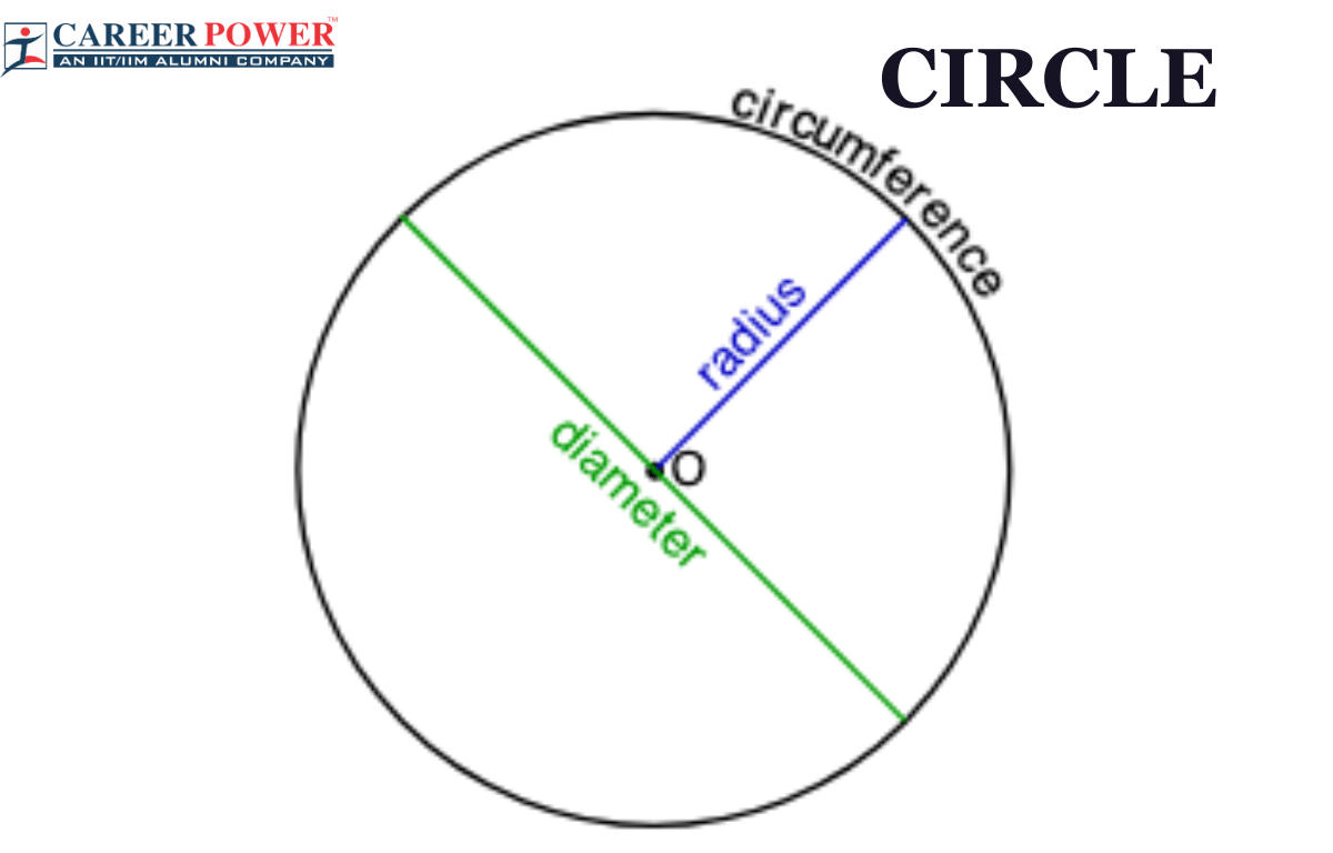
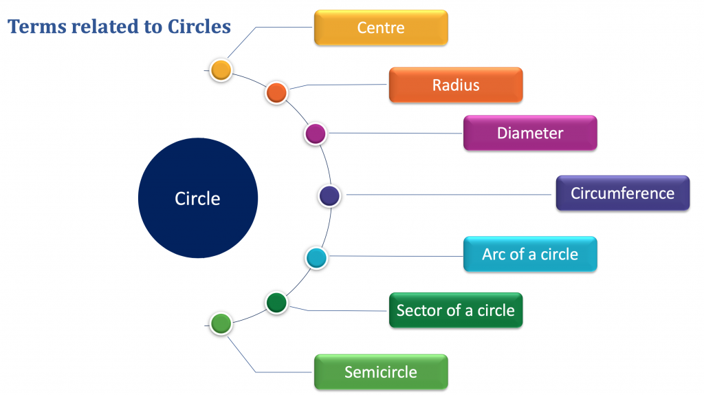
Circle Properties
Circles have several key properties. The radius (r) is the distance from the center to any point on the circle. The diameter (d) is twice the radius (d = 2r). The circumference (C) is the distance around the circle, calculated as C = 2πr or C = πd. The area (A) enclosed by the circle is A = πr².
A sector is a portion of a circle enclosed by two radii and an arc; its area is (θ/360°)πr², where θ is the central angle in degrees. A segment is the area between a chord and the arc it subtends. Arc length is a portion of the circumference, calculated as (θ/360°)2πr. All these measurements are typically expressed in units of length (e.g., meters, centimeters) or area (e.g., square meters, square centimeters).
Real-World and Abstract Examples of Circles
Circles pop up everywhere,
asli*. Here are some examples
- A bicycle wheel (a very close approximation): The wheel’s circular shape allows for smooth rotation.
- A coin (a close approximation): The near-perfect circular shape facilitates easy handling and stacking.
- The orbit of a planet around a star (an approximation): Planetary orbits are elliptical, but often approximated as circles for simplification.
- A pizza (a close approximation): The circular shape allows for even cooking and easy slicing.
- A ripple in a pond after dropping a stone (a close approximation): The expanding circular wave demonstrates circular symmetry.
Abstract examples include:
- The unit circle in trigonometry: A circle with radius 1, used to define trigonometric functions.
- The circle group in abstract algebra: A group formed by rotations of a circle.
- Circular functions in calculus: Functions such as sine and cosine are intrinsically linked to the unit circle.
Circle Theorems
Several theorems describe the properties of circles.
- Thales’ Theorem: If A, B, and C are points on a circle where the line AC is a diameter, then the angle ∠ABC is a right angle (90°).
-(Imagine a right-angled triangle perfectly inscribed within a semicircle)* - Inscribed Angle Theorem: An inscribed angle is half the measure of the central angle that subtends the same arc.
-(Picture an angle formed by two chords meeting on the circle’s circumference. The angle’s measure is half the angle at the circle’s center subtending the same arc.)* - Power of a Point Theorem: For a point P outside a circle, the product of the lengths of the two segments from P to the circle along any line through P is constant.
-(Envision a line intersecting a circle at two points. The product of the distances from the external point to those intersection points is constant regardless of the line’s angle.)*
Comparative Analysis: Circle vs. Ellipse
| Feature | Circle | Ellipse |
|---|---|---|
| Definition | Set of points equidistant from a center | Set of points such that the sum of distances to two foci is constant |
| Equation | (x – a)² + (y – b)² = r² | (x²/a²) + (y²/b²) = 1 |
| Eccentricity | 0 | 0 < e < 1 |
| Foci | One point (center) | Two points |
| Major/Minor Axis | Equal (diameter) | Unequal (major and minor axes) |
The Concept of Infinity
Euy, so we’ve talked about circles, aye? Now, let’s get into the
real* mind-bending stuff
infinity. It’s not just a big number, ah, it’s a whole different level of
edan*, you know? Think of it like this
the number of grains of sand on a beach – massive, right? But infinity is way beyond that, it’s like,
jauh banget* beyond comprehension.
Infinity in math isn’t just one thing; it’s got different flavors, man. It’s like choosing between different
-mie ayam* – some are spicy, some are savory, some are
-pedes banget*. We’re dealing with different
-kinds* of infinity, each with its own unique properties. And understanding these different types is crucial when we start thinking about circles and their properties.
Types of Infinity
There are different sizes of infinity, it’s not all the same. Some infinities are “bigger” than others. It sounds crazy,
- tau*, but it’s true! Think of it like comparing the number of stars in the sky versus the number of grains of sand on Earth. Both are huge, but one might be
- way* bigger. This is where the concept of countable and uncountable infinities comes in.
Countable vs. Uncountable Infinity
Imagine you’re counting numbers, 1, 2, 3… You can, theoretically, keep going forever, right? That’s countable infinity. The set of all natural numbers (1, 2, 3…) is infinitely large, but it’s still “countable” because you can, in principle, assign each number a unique position in a sequence.
Gak pake mikir keras banget, kan?*
Now, imagine trying to count all the points on a line segment. You can’t! No matter how small a step you take, there are always infinitely many points between any two points you choose. This is uncountable infinity, which is a “bigger” infinity than the countable one. It’s like trying to count all the
gorengan* sold in Bandung – impossible!
Limits and Circles
Think about the circumference of a circle. As you increase the number of sides of a polygon inscribed within the circle, the polygon gets closer and closer to the circle. The perimeter of the polygon approaches the circumference of the circle. This “approaching” is what limits are all about. It’s like chasing a
- angkot* – you get closer and closer, but you might never
- exactly* reach it. The limit represents the value the polygon’s perimeter approaches as the number of sides goes to infinity. In this case, the limit is the circle’s circumference.
- Asyik, kan?*
Points on a Circle’s Circumference
Euy, so we’re diving deep into the
- misterius* world of circles, specifically, the points on its edge, lah. It’s a bit of a mind-bender, but stick with me, ya? We’ve already talked about infinity, and now we’re gonna see how that relates to something seemingly simple like a circle. Aduh, it’s gonna be
- a bit of a trip*.
The number of points on a circle’s circumference is,
- get this*, infinite. Yeah, you heard me right –
- infinite*. It’s not like you can count them one by one,
- ngarampas*! This is because a circle is a continuous curve; there are no gaps or breaks. Between any two points on the circumference, you can always find another point. This is where the concept of infinity comes into play – you can keep subdividing the space between any two points endlessly. It’s like zooming in on a photo; no matter how much you zoom, you’ll always find more detail.
It’s
- amazing*, right?
The Density of Points on a Circle’s Circumference
This infinite nature of points means that the density of points is also infinite. Imagine trying to measure the distance between two points on the circumference – you can always find a point in between. The more you zoom in, the more points you seem to discover. It’s like those fractal patterns –
- amazing*,
- kan?*
Visual Representation of Point Density
To illustrate this, imagine a simple visual representation. We’ll use a table to show how the apparent number of points increases with magnification. Picture a circle. First, we look at it with the naked eye – we might see a smooth curve, and it looks like there are only a few noticeable points. Then, we zoom in with a magnifying glass.
Now, we see more detail, and it seems like there are more points. If we could use a super-powerful microscope, we’d see evenmore* points. This process could continue indefinitely, highlighting the infinite nature of the points.
| Magnification | Apparent Number of Points |
|---|---|
| Naked Eye | Few (appears smooth) |
| 10x Magnification | Many more points visible |
| 100x Magnification | Significantly more points, almost uncountable |
| 1000x Magnification | Appears densely packed with points; practically infinite |
This table is a
- simplified* representation, of course. The actual number of points is always infinite, regardless of the magnification. It’s just to give you a
- feel* for the concept. It’s like trying to count the grains of sand on a beach – you can count some, but the total is
- impossible* to determine because it’s so vast.
Circle’s Perimeter and its Implications
Nah, so we’ve talked about circles and infinity, now let’s get into the nitty-gritty of measuring their,ahem*, girth. We’re diving into the circumference – the distance around a circle. It’s all tied up with pi, that crazy irrational number, and it gets pretty mind-bending.
Formula and Calculation
Calculating a circle’s circumference is pretty straightforward,
asal* you remember the formulas. It’s all about using pi (π), which is approximately 3.14159, and either the diameter (d) or the radius (r). The radius is the distance from the center to the edge, and the diameter is twice the radius. Here’s the lowdown
| Formula | Description |
|---|---|
| C = πd | Circumference using diameter |
| C = 2πr | Circumference using radius |
Let’s do some calculations, – ya*.First, let’s find the circumference of a circle with a radius of 5 cm. Using the formula C = 2πr, we get: C = 2
- π
- 5 cm = 10π cm ≈ 31.4159 cm. So, the circumference is approximately 31.42 cm.
Now, for a circle with a diameter of 12 inches. Using C = πd, we have: C = π
- 12 inches ≈ 37.6991 inches. Rounding it off, we get a circumference of approximately 37.70 inches.
- Gampang banget, kan?*
Circumference and the Concept of Infinity
The relationship between a circle’s circumference and pi is,ealah*, deeply intertwined. Pi is irrational, meaning its decimal representation goes on forever without repeating.
The infinite nature of π directly implies that the precise circumference of any circle with a non-zero radius cannot be exactly calculated using finite methods. You can get closer and closer, but you’ll never quite hit the mark.
This infinite decimal expansion of π means that no matter how many decimal places you use in your calculations, you’re still only getting an approximation of theactual* circumference. It’s like chasing a shadow – you can get close, but never truly catch it.
Precision of Measurement and Perceived Length
Increasing the precision of our measurement tools (like going from centimeters to millimeters to micrometers) only changes the number of decimal places in our circumference calculation. For example, if we use a more precise value of π (say, 3.14159265359), the circumference of our 5 cm radius circle becomes more precise, but it still won’t beexactly* right. It’s still an approximation.The irrationality of π fundamentally limits our ability to determine the “true” circumference.
We can get incredibly close, but true precision is impossible.In the real world, this has practical implications. In engineering, the level of precision needed varies greatly depending on the application. Building a bridge requires far more precise measurements than, say, making a pizza. Similarly, in astronomy, measuring the circumference of a planet or star requires incredibly sophisticated techniques and tools, but even then, there will always be a margin of error due to the nature of π.
Infinite Series and Circles
Aduh, ngomongin lingkaran sama deret tak hingga? Enaknya, nih! Kayak lagi ngopi di Angkringan, santai tapi penuh wawasan. Kita bakal liat gimana deret tak hingga bisa bantu kita ngitung keliling lingkaran, walaupun lingkaran itu sendiri bentuknya,ehem*, tak terbatas. Pokoknya, siap-siap melek mata, ya!
Infinite series, atau deret tak hingga dalam bahasa kita, itu sederet angka yang jumlahnya terus berlanjut tanpa henti. Bayangin aja kayak ngitung butiran pasir di pantai – nggak akan selesai-selesai! Nah, deret ini bisa kita pake buat ngedekati nilai keliling lingkaran. Kenapa? Karena keliling lingkaran itu sendiri melibatkan angka π (pi), yang nilainya irrasional, artinya angka di belakang koma itu nggak pernah berhenti.
Jadi, deret tak hingga jadi alat bantu yang cukup ampuh untuk mendapatkan perkiraan yang akurat.
Approximating Circumference Using Infinite Series
Salah satu cara paling terkenal untuk ngitung π (dan otomatis keliling lingkaran) adalah pake deret Leibniz. Deret ini nyajikan π sebagai jumlah dari deret tak hingga yang melibatkan pecahan. Rumusnya gini:
π/4 = 1 – 1/3 + 1/5 – 1/7 + 1/9 – …
Semakin banyak suku yang kita jumlahkan, semakin akurat pendekatan kita terhadap nilai π. Tapi, perlu diingat, ya, ini cuma pendekatan. Nggak bakal pernah persis sama, karena π itu sendiri nggak bisa diwakilin dengan angka yang pas.
Examples of Relevant Infinite Series
Selain deret Leibniz, ada beberapa deret tak hingga lain yang bisa dipake buat ngitung π. Misalnya, ada deret Gregory-Leibniz (sama aja sebenernya dengan Leibniz), terus ada deret Nilakantha, dan masih banyak lagi. Masing-masing punya tingkat konvergensi yang berbeda-beda. Konvergensi itu seberapa cepet deret tersebut mendekati nilai sebenarnya.
Comparison of Different Infinite Series Methods
Nah, sekarang kita banding-bandingin. Deret Leibniz, misalnya, konvergensinya agak lambat. Artinya, kita perlu jumlahin banyak banget suku buat dapetin nilai π yang akurat. Sementara deret Nilakantha, konvergensinya lebih cepet. Jadi, dengan jumlah suku yang lebih sedikit, kita udah bisa dapetin pendekatan yang lebih akurat.
Ini semua tergantung seberapa akurat kita pengen dapetin nilai π-nya. Kayak milih nasi goreng, ada yang pedes banget, ada yang sedang, ada yang nggak pedes sama sekali, tergantung selera, gitu!
Circle’s Area and Infinity
Euy, so we’ve been geeking out about circles and infinity, right? We’ve talked about the points on the circumference – a whole lotta’ them! Now, let’s dive into the area – it’s another wild ride with infinity. Think of it as the
- isi* (filling) of the circle, not just the
- pinggir* (edge).
The area of a circle, man, it’s like a magical formula that connects the radius to the total space inside. It’s all about thatluas*, you know? It’s a fundamental concept in geometry, and it’s got a surprising connection to infinity.
Calculating a Circle’s Area
The formula for calculating a circle’s area is famously simple, but powerful:
Area = πr²
where ‘r’ is the radius (the distance from the center to the edge) and π (pi) is that ever-elusive, irrational constant, approximately 3.14159. This formula tells us how much space the circle occupies. It’s a straightforward calculation, but the implications are mind-bending when you consider infinity.
The Relationship Between Area and Infinity
The relationship between a circle’s area and infinity is subtle but significant. As the radius (r) of a circle increases, the area (πr²) increases proportionally to the square of the radius. This means that even small increases in the radius lead to significantly larger increases in the area. This isn’t just a linear increase; it’s exponential growth! Think about it: a tiny increase in radius can lead to a huge jump in area, highlighting the ever-expanding nature of the area as the radius grows towards infinity.
It’s like, the bigger the circle, the more
edan* (crazy) the area gets!
Visual Representation of Increasing Circle Area
Imagine we start with a small circle, maybe the size of a coin.
Imagine a small circle, like a Rp 1000 coin. Its area is relatively small.
Now, let’s increase the radius. Maybe we make it the size of a dinner plate. The area has increased considerably!
Now, imagine the circle is as big as a dinner plate. The area has significantly increased compared to the coin.
Let’s go bigger! Let’s say we make it the size of a large pizza. The area is now huge!
Now imagine the circle as large as a pizza. The increase in area is dramatic!
Keep going! Imagine a circle the size of a swimming pool, then a lake, then an ocean… The area keeps increasing, approaching infinity as the radius increases without bound. The space inside the circle becomes astronomically vast. It’s like,
wah gila* (wow crazy), right?
Geometric Series and Circles

Euy, urang bahas hubungan geometrik seri jeung lingkaran, nya! Kitu lho, ternyata konsep matematika nu ketokna jauh beda teh bisa dihubungkeun. Asik pisan, lah!
Geometric series, eta runtunan angka dimana tiap suku dikalikeun ku angka konstanta (rasio) pikeun meunangkeun suku salajengna. Lingkaran mah, hayu urang inget-inget deui, bentuk geometrik dua dimensi jeung titik-titik nu jarakna sarua ka titik tengah (pusat lingkaran). Nah, hubungan dua konsep ieu rada unik, tapi bisa dijelaskeun ku cara nu gampang dipahami, kok!
Geometric Series Definition and Circle Properties
Hayu urang jelaskeun dulu definisi geometrik seri jeung sifat-sifat lingkaran. Ieu penting pisan supaya urang bisa ngarti hubungan di antara dua hal ieu.
Geometric Series: Suatu deret geometrik didefinisikan sebagai jumlah suku-suku dalam suatu barisan geometrik. Suku ke-n (a n) dari deret geometrik diberikan oleh rumus:
an = ar n-1
dimana ‘a’ adalah suku pertama dan ‘r’ adalah rasio umum (rasio antar suku). Jumlah n suku pertama (S n) dari deret geometrik adalah:
Sn = a(1 – r n) / (1 – r)
, asalkan r ≠ 1. Deret geometrik konvergen jika |r| < 1, dan jumlah tak hingga nya adalah
S∞ = a / (1 – r)
. Mun |r| ≥ 1, deret geometrik divergen, hartina jumlahna teu terbatas.
Circle Properties: Lingkaran dicirikeun ku radius (r), diameter (d = 2r), keliling (C = 2πr), jeung luas (A = πr²).
(Diagram: A circle with radius ‘r’, diameter ‘d’ marked, and an arc showing a segment) Bayangkeun hiji lingkaran, garis tengahna (diameter) nyambungkeun dua titik paling jauh dina lingkaran, ngaliwatan titik tengahna. Radius nyaeta garis lurus ti titik tengah ka sembarang titik dina keliling lingkaran. Keliling teh panjang garis lengkung nu ngawatesan lingkaran, sedengkeun luas teh daerah nu diwatesan ku keliling lingkaran.
Connecting Geometric Series and Circles: Geometric series bisa dipaké pikeun ngira-ngira atawa ngamodelkeun aspek-aspek perhitungan lingkaran, utamana nu patali jeung pendekatan nilai π atawa perhitungan luas segmen lingkaran. Contohna, rumus Leibniz pikeun π ngagunakeun deret geometrik.
Approximating π using Leibniz Formula
Rumus Leibniz pikeun π mangrupa conto anu paling dikenal kumaha deret geometrik bisa dipaké pikeun ngira-ngira nilai π. Rumusna nyaéta:
π/4 = 1 – 1/3 + 1/5 – 1/7 + 1/9 – …
Lamun urang ngitung jumlah sababaraha suku awal deret ieu, urang bakal meunangkeun pendekatan nilai π. Misalna, lamun urang ngagunakeun 100 suku pertama, urang bakal meunangkeun pendekatan π nu lumayan akurat, sanajan teu persis.
Contona, lamun urang ngitung lima suku pertama, urang bakal meunang: 1 – 1/3 + 1/5 – 1/7 + 1/9 ≈ 0.7604. Kalikeun ku 4, urang meunang pendekatan π ≈ 3.0416. Sedengkeun nilai π sebenarnya kira-kira 3.14159. Semakin banyak suku yang digunakan, semakin akurat pendekatannya.
Calculating Areas of Circular Segments using Geometric Series
Hayu urang bayangkeun hiji segmen lingkaran, eta bagian lingkaran nu diwatesan ku dua jari-jari jeung busur lingkaran. Dina kasus anu sederhana, luas segmen lingkaran bisa dihitung ku cara ngurangan luas segitiga anu dibentuk ku dua jari-jari jeung tali busur ti luas sektor lingkaran anu dibentuk ku dua jari-jari jeung busur.
(Diagram: A circular segment with radius ‘r’, central angle θ, and segment area shaded.) Dina kasus anu leuwih kompleks, metode numerik anu ngagunakeun deret geometrik bisa dipaké pikeun ngira-ngira luas segmen lingkaran.
(A step-by-step calculation example would be provided here, demonstrating how a geometric series could be applied, although it might be complex and beyond the scope of a simple explanation without extensive mathematical formulas.)
Modeling Circular Motion using Geometric Series
Bayangkeun hiji titik nu gerak melingkar, tapi jarakna ka titik tengah na jadi leutik terus-terusan dina unggal puteran. Jarak nu ditempuh dina unggal puteran bisa dimodelkeun ku deret geometrik. Contona, lamun jarak dina puteran kahiji nyaéta ‘d’, jeung jarakna jadi satengahna dina unggal puteran salajengna, maka jarak total nu ditempuh bisa diitung ku rumus jumlah deret geometrik tak hingga.
(A detailed calculation showing how a geometric series models the total distance covered in this scenario would be presented here.)
Comparison of Geometric Series Types
Ayeuna, urang bandingkeun dua tipe deret geometrik anu bisa dipaké dina perhitungan lingkaran: deret geometrik hingga jeung deret geometrik tak hingga.
| Feature | Geometric Series Type 1: Finite Geometric Series | Geometric Series Type 2: Infinite Converging Geometric Series |
|---|---|---|
| Formula | Sn = a(1 – rn) / (1 – r) | S∞ = a / (1 – r) (|r| < 1) |
| Convergence | Always converges (finite sum) | Converges if |r| < 1 |
| Application to Circles | Approximating π or areas with a specified number of terms | Approximating π or other circular properties with potentially higher accuracy |
| Advantages | Simple calculation, always yields a result | Potentially higher accuracy with fewer terms if convergent |
| Disadvantages | Accuracy depends on the number of terms; can be less accurate for fewer terms | Only applicable if |r| < 1; can be slow to converge |
Error Analysis of π Approximation
Lamun urang ngagunakeun deret Leibniz pikeun ngira-ngira π, aya kasalahan nu bakal timbul kusabab urang ngan ukur ngagunakeun sababaraha suku awal. Kasalahan ieu bakal turun lamun jumlah suku nu dipaké leuwih loba.
(A table or graph showing the error in the approximation of π as a function of the number of terms used in the Leibniz formula would be presented here.)
Fractal Geometry and Circles
Euy, so we’ve been geeking out about circles and infinity, kan? Now, let’s add some
serious* mind-bending stuff
fractal geometry. Think of it as the ultimate “infinite detail” game – zooming in reveals more and more complexity, just like those never-ending patterns on a mandala, tau?Fractal geometry shows how infinity can manifest within a seemingly simple shape like a circle. It’s all about self-similarity – smaller parts of the pattern look just like the bigger picture, only smaller.
This repetition at different scales creates this awesome, infinite detail. Aduh, bikin kepala pusing, tapi keren banget!
Self-Similar Patterns in Circular Fractals
The beauty of fractal geometry lies in its ability to generate infinitely complex patterns within a finite space, such as a circle. Imagine a circle divided into segments, each segment further divided into smaller segments, and so on ad infinitum. This process creates a pattern that repeats itself at increasingly smaller scales. This self-similarity is the hallmark of fractal geometry.
We can see this in nature, too – think of the spirals in a nautilus shell or the branching patterns of a tree. It’s the same concept, only applied to a circle.
The Mandelbrot Set and Circular Representation
While the Mandelbrot set itself isn’t strictly a circle, its representation can be confined within a circular boundary. The incredibly intricate patterns within the Mandelbrot set demonstrate the concept of infinite detail. Zooming in reveals ever-more complex structures, showcasing the self-similarity characteristic of fractals. This highlights how even within a bounded space (our circle), infinite complexity can be generated.
The intricate patterns could be mapped onto a circle, with different regions of the circle representing different sections of the Mandelbrot set.
Visual Representation of a Circular Fractal
Imagine a circle. Now, imagine dividing that circle into four equal quadrants. Each quadrant is then divided into four smaller quadrants, and so on, infinitely. Each division creates a smaller circle within a circle.
This recursive process generates an infinitely complex pattern within the original circle. The pattern is self-similar, meaning each smaller circle exhibits the same structure as the larger circle. It’s like a never-ending Russian nesting doll, but infinitely detailed and stunningly beautiful.
The visual representation would show concentric circles, each progressively smaller, creating a visually captivating display of infinite complexity contained within a finite boundary. The color of each circle could vary to emphasize the self-similarity and the recursive nature of the pattern. It’s like a cosmic kaleidoscope, a visual representation of infinity within a circle.
Limits and Approximations
Eh, so we’ve been messing around with circles and infinity, right? Now, let’s get a bit more
- mathematic* and talk about how we can actually
- deal* with those infinite things in a practical way. We’re gonna use
- limits* – think of it as sneaking up on infinity without actually getting there,
- a la* slow-motion chase scene in a FTV.
Basically, limits are all about approaching a value as closely as you want, without necessarily ever reaching it. It’s like aiming for that perfect cup of kopi tubruk – you’ll never quite get it
-exactly* right, but you can get
-damn* close.
Formal Definition and Application to Circles
The formal definition of a limit uses the epsilon-delta notation. It’s a bit
-gembel*, but bear with me. For a function f(x), we say that the limit of f(x) as x approaches ‘a’ is L (written as lim x→a f(x) = L) if for every ε > 0, there exists a δ > 0 such that if 0 < |x - a| < δ, then |f(x)
-L| < ε. Basically, we can make f(x) as close to L as we want (within ε) by making x sufficiently close to a (within δ).
This applies to circles because π, the ratio of a circle’s circumference to its diameter, is irrational – it goes on forever without repeating. We can’t
-exactly* calculate the circumference or area, but we can use limits to get arbitrarily close. Imagine a circle with inscribed and circumscribed regular polygons. As the number of sides of the polygons increases, their perimeters and areas get closer and closer to the circle’s actual circumference and area.
The limit of the perimeters and areas of these polygons, as the number of sides approaches infinity, gives us the circle’s circumference and area.
Imagine a diagram: a circle with a square inside it (inscribed) and a square around it (circumscribed). Then, replace the squares with octagons, then hexadecagons, and so on. Each time, the polygons get closer to the circle’s shape, their perimeters and areas getting closer to the circle’s actual values. The limit of this process gives us the exact values, even though π is irrational.
Approximation Methods using Limits
There are several ways to approximate a circle’s properties using limits, each with its own strengths and weaknesses. Think of it like choosing the right
-gojek* driver – some are fast, some are cheap, some are both…rarely!
The method of exhaustion is a classic. We approximate the circle’s area by using the areas of inscribed and circumscribed polygons. Let’s say we start with a square (4 sides). Then, we double the number of sides to get an octagon (8 sides), then a 16-sided polygon, and so on. As the number of sides increases, the area of the polygons converges to the area of the circle.
For example, let’s say the circle has a radius of 1. The area of the inscribed square is 2, and the circumscribed square’s area is 4. With an octagon, the areas get closer to π (approximately 3.14159). This process continues, refining the approximation with each iteration.
Limits are also used to derive the circumference formula (C = 2πr). Imagine dividing the circumference into infinitely small arcs. Each arc can be approximated as a straight line segment. Summing up the lengths of these segments using integration (which is fundamentally based on limits) gives us the total circumference.
Taylor series expansions are another powerful tool. We can use infinite series to approximate π. For instance, the Leibniz formula for π is given by: π/4 = 1 – 1/3 + 1/5 – 1/7 + … Another series is the Nilakantha series: π = 3 + 4/(2*3*4)
-4/(4*5*6) + 4/(6*7*8)
-… These series converge to π, allowing us to approximate the circumference and area.
Comparative Analysis of Approximation Methods
Here’s a quick rundown comparing the methods, think of it like comparing
-mie ayam* from different stalls – each has its own
-rasa* (taste) and
-harga* (price):
| Method | Description | Advantages | Disadvantages | Convergence Rate |
|---|---|---|---|---|
| Method of Exhaustion | Approximating area using inscribed/circumscribed polygons. | Simple conceptually, geometrically intuitive. | Slow convergence, computationally intensive for high accuracy. | Relatively Slow |
| Taylor Series Expansion (e.g., Leibniz formula for π) | Using infinite series to approximate π. | Relatively fast convergence for some series. | Requires knowledge of calculus and series expansion. | Moderate to Fast |
| Monte Carlo Method | Randomly sampling points within a square containing a circle. | Simple to implement, parallelizable. | Slow convergence, accuracy depends on the number of samples. | Slow |
Error Analysis
Estimating the error in these approximations is crucial. It’s like knowing how much
-salah* (error) you’re making in your
-resep* (recipe)!
For the method of exhaustion, the error decreases as the number of polygon sides increases. A graph would show the error decreasing exponentially. For Taylor series, the error is related to the remainder term of the series, which gets smaller as more terms are included. A graph would show the error decreasing as the number of terms increases.
The Monte Carlo method’s error decreases with the square root of the number of samples; a graph would show a gradual decrease.
Practical Applications
Approximating circle properties is
-super* important in many fields. Think of engineering designs, physics calculations, and even baking a perfect round cake!
In engineering, accurate calculations are essential for things like designing circular pipes, gears, or wheels. In physics, circular motion is everywhere, from planets orbiting stars to electrons orbiting nuclei. The accuracy of these approximations directly impacts the reliability and performance of these systems. However, computational limitations and the required accuracy often restrict the choice of approximation method in practical scenarios.
Advanced Considerations
The relationship between limits and derivatives is also important. The derivative of the area of a circle with respect to its radius is the circumference, demonstrating a fundamental connection between these concepts. Infinitesimal quantities, though conceptually challenging, provide an intuitive way to understand limits and their application in approximating circular properties.
Pi and its Infinite Nature
Euy, so we’ve been geeking out about circles, right? Now, let’s talk about the real MVP of the circle world: Pi (π). This ain’t just some random number, ah? It’s the ratio of a circle’s circumference to its diameter – and that’s where things get
super* interesting.
Pi is famously irrational, meaning its decimal representation goes on forever without repeating. This infinite nature is what makes calculating things related to circles so… well,complicated*. Think of it like trying to count all the grains of sand on a beach – you can keep going and going, but you’ll never reach the end. That’s Pi in a nutshell, man.
Okay, so the whole “does a circle have infinite points?” thing is kinda mind-bending, right? It’s like thinking about the triarchic theory of intelligence; to understand that, you should check out who developed the triarchic theory of intelligence , which is pretty complex itself. Anyway, back to circles – that infinite point thing is a similar brain-teaser, all about limits and how we define things mathematically.
Pi’s Properties and Relationship to the Circle
Pi’s value is approximately 3.14159, but that’s just scratching the surface. Its relationship with circles is fundamental; it’s the constant that links a circle’s diameter to its circumference. The formula, C = πd (where C is the circumference and d is the diameter), is a cornerstone of geometry. Without Pi, we’d be completely lost when dealing with circles’ perimeters, areas, and volumes of related shapes like spheres and cylinders.
It’s the key ingredient, man!
Implications of Pi’s Infinite Decimal Representation
The fact that Pi’s decimal representation is infinite means we can only ever approximate its value. We can use more and more decimal places for greater accuracy, but we’ll never reach a perfectly precise representation. This has implications for precision in engineering, architecture, and other fields where precise circle calculations are crucial. Imagine building a giant Ferris wheel – you need Pi to be as accurate as humanly possible! A tiny error in Pi can lead to a noticeable difference in the final product.
Impact of Pi’s Infinite Nature on Circle Calculations
Let’s say you’re trying to calculate the area of a pizza (a circle, obviously). The formula is A = πr² (where A is the area and r is the radius). Using a truncated value of Pi, like 3.14, will give you an approximation. The more decimal places of Pi you use, the closer your calculated area will be to the true area.
However, you’ll never get a perfectly accurate answer because Pi’s infinite. It’s like trying to perfectly measure something with a ruler that has infinitely small gradations. You can get close, but never exact.
Trigonometry and Circles: Does A Circle Have Infinte Theory
Aduh, trigonometry and circles, eh? Sounds like a pretty
- nyunda* (challenging) topic, but
- tenang aja* (calm down), we’ll break it down
- sunda style* (Bandung style). It’s all about how angles and lengths on a circle relate to those trigonometric functions you’ve probably been wrestling with. Think of it as a
- ngaliwet* (cozy) dance between geometry and algebra.
Trigonometric Functions and the Unit Circle
The unit circle, a circle with a radius of 1, is thejantung hati* (heart) of this whole thing. Any point on the unit circle’s circumference can be described using its angle (θ) from the positive x-axis and its x and y coordinates. These coordinates are directly related to the cosine and sine of the angle, respectively. The cosine (cos θ) is the x-coordinate, and the sine (sin θ) is the y-coordinate.
The tangent (tan θ) is the ratio of sine to cosine (sin θ / cos θ). Imagine a right-angled triangle formed by the origin, the point on the circle, and the projection of that point onto the x-axis. The hypotenuse is the radius (1), the adjacent side is cos θ, and the opposite side is sin θ.
Examples of Trigonometric Applications in Circle Calculations
Here are some
praktis* (practical) examples to show how useful this relationship is
- Finding the Area of a Sector: Let’s say we have a circle with a radius of 5 cm and a sector with a central angle of 60 degrees. To find the area of the sector, we use the formula: Area = (θ/360)
πr², where θ is the angle in degrees and r is the radius. Plugging in our values, we get
Area = (60/360)
- π
- 5² = (1/6)
- 25π ≈ 13.09 cm².
- Calculating the Length of an Arc: Consider a circle with a radius of 10 meters and an arc subtended by a central angle of 45 degrees. The arc length is calculated using the formula: Arc length = (θ/360)
2πr. Converting 45 degrees to radians (π/4), we have
So, does a circle have infinite points? It’s a pretty mind-bending question, right? Thinking about it makes me wonder about other infinite systems, like the craziness described in this article comparing different chaotic systems: is jwcc chaos theory big eatie bigger then jwd rexy. The sheer scale of that comparison makes the infinite points of a circle seem almost manageable in comparison.
Ultimately, the infinity of a circle’s points is a different kind of infinity than the potentially infinite complexity of those chaotic systems.
Arc length = (π/4)
- 2π
- 10 = 5π meters ≈ 15.71 meters.
- Determining the Coordinates of a Point: Suppose a point lies on a circle with a radius of 8 units at an angle of 120 degrees. To find its coordinates, we use: x = r
- cos θ and y = r
- sin θ. Therefore, x = 8
- cos(120°) = -4 and y = 8
- sin(120°) = 4√3. The coordinates of the point are (-4, 4√3).
Comparison of Trigonometric Functions and Their Relation to Circles
Here’s a table summarizing the six trigonometric functions:
| Function | Right-Angled Triangle Definition | Unit Circle Definition | Relationship to Circle Properties |
|---|---|---|---|
| Sine (sin θ) | Opposite/Hypotenuse | y-coordinate | Relates the y-coordinate of a point on the unit circle to the angle. |
| Cosine (cos θ) | Adjacent/Hypotenuse | x-coordinate | Relates the x-coordinate of a point on the unit circle to the angle. |
| Tangent (tan θ) | Opposite/Adjacent | y-coordinate/x-coordinate | Slope of the line connecting the origin to the point on the unit circle. |
| Cosecant (csc θ) | Hypotenuse/Opposite | 1/y-coordinate | Reciprocal of sine; related to the y-coordinate. |
| Secant (sec θ) | Hypotenuse/Adjacent | 1/x-coordinate | Reciprocal of cosine; related to the x-coordinate. |
| Cotangent (cot θ) | Adjacent/Opposite | x-coordinate/y-coordinate | Reciprocal of tangent; related to the slope. |
Radians are a measure of angles where one radian is the angle subtended at the center of a circle by an arc equal in length to the radius. Using radians simplifies many trigonometric calculations, especially those involving calculus, because they directly relate the angle to the arc length. It eliminates the need for conversion factors like π/180 that are necessary when using degrees.
Geometric Representation of the Pythagorean Identity
The Pythagorean identity, sin²θ + cos²θ = 1, is a beautiful geometric truth. On the unit circle, it simply states that the sum of the squares of the x and y coordinates of any point on the circle equals the square of the radius (which is 1). Imagine a right-angled triangle formed by the origin, the point on the circle, and the projection of that point onto the x-axis.
The Pythagorean theorem (a² + b² = c²) directly translates to sin²θ + cos²θ = 1.(Simple diagram: A unit circle with a point (x,y) on the circumference. A right-angled triangle is drawn with the hypotenuse as the radius from the origin to the point (x,y), the adjacent side along the x-axis, and the opposite side parallel to the y-axis.
x represents cos θ and y represents sin θ.)
Real-World Applications of Trigonometry and Circles
Understanding the relationship between trigonometry and circles is
penting banget* (very important) in many fields
- Navigation: Determining distances and bearings using angles and distances. Think GPS!
- Engineering: Designing circular structures like bridges, tunnels, and gears.
- Physics: Analyzing circular motion, like the movement of planets or a spinning top.
- Computer Graphics: Creating and manipulating circular and curved shapes in 2D and 3D.
- Astronomy: Calculating planetary orbits and celestial positions.
Handling Angles Greater Than 360 Degrees or Negative Angles
Angles greater than 360 degrees or negative angles simply represent multiple rotations around the unit circle. For example, an angle of 420 degrees is equivalent to 360 + 60 degrees, meaning it’s the same point on the unit circle as a 60-degree angle. Similarly, a -30-degree angle is the same as a 330-degree angle. The trigonometric function values repeat every 360 degrees (or 2π radians).
Inverse Trigonometric Functions and Their Geometric Interpretation
Inverse trigonometric functions (arcsin, arccos, arctan) find the angle whose sine, cosine, or tangent is a given value. Geometrically, on the unit circle, arcsin(x) gives the y-coordinate, arccos(x) gives the x-coordinate, and arctan(x) gives the ratio of y/x. Their domains and ranges are restricted to ensure a single, unambiguous angle is returned.
Determining the Equation of a Circle Using Trigonometric Functions
The equation of a circle with center (h, k) and radius r is (x – h)² + (y – k)² = r². We can also express this using trigonometric functions: x = h + r cos θ and y = k + r sin θ, where θ is the angle. For example, a circle centered at (2, 3) with a radius of 4 has the equation (x – 2)² + (y – 3)² = 16, and parametrically x = 2 + 4 cos θ and y = 3 + 4 sin θ.
Calculus and Circles
Nah, so we’ve been exploring circles and infinity, right? Now, let’s crank it up a notch and see how calculus, that
- sangat* powerful tool, helps us understand circles even better. It’s like adding extra
- bumbu* to an already delicious dish! We’ll be looking at how integral and differential calculus can be used to solve problems related to circles, from finding areas and arc lengths to tackling optimization and related rates. Prepare for some serious
- kekinian* math!
Circumference and Arc Length
Calculating the circumference of a circle using calculus involves integrating the infinitesimal arc lengths along the circle’s perimeter. The formula for the circumference (C) of a circle with radius r is derived by integrating the arc length element along the circumference. The integral represents the sum of infinitely small arc lengths.
C = ∫02π r dθ = 2πr
For arc length (s) of a circle segment subtended by a central angle θ (in radians) and radius r:
s = rθ
Example 1: A circle has a radius of 5 cm. Find its circumference. Using the formula, C = 2π(5) = 10π cm.Example 2: A circle has a radius of 7.2 meters. Find the arc length subtended by a central angle of π/3 radians. Using the formula, s = 7.2 – (π/3) = 2.4π meters.
Area of a Circle and Circular Segments
The area of a circle can be derived using both single and double integration. Single integration involves integrating the area of infinitely thin concentric rings, while double integration considers the area element in polar coordinates.Using single integration:
A = ∫0r 2πx dx = πr²
Using double integration:
A = ∫02π ∫ 0r r dr dθ = πr²
To calculate the area of a circular segment, we need to consider the area of the sector and the area of the triangle formed by the two radii and the chord. The area of a circular segment is given by:
Asegment = (1/2)r²(θ – sinθ)
where θ is the central angle in radians.Example: Find the area of a sector of a circle with radius 10 cm and a central angle of π/4 radians. The area is (1/2)(10)²(π/4) = 25π/2 cm².
Tangents and Normals
Finding the equation of the tangent and normal lines to a circle at a given point uses differential calculus. For a circle with equation x² + y² = r², the slope of the tangent at (x 0, y 0) is given by implicit differentiation:
2x + 2y(dy/dx) = 0 => dy/dx = -x/y
The equation of the tangent line is then:
y – y0 = (-x 0/y 0)(x – x 0)
The normal line is perpendicular to the tangent line, so its slope is the negative reciprocal of the tangent’s slope.Example: Find the equation of the tangent and normal lines to the circle x² + y² = 25 at the point (3, 4).
Optimization Problems
Optimization problems involving circles often involve finding maximum or minimum values. A classic example is finding the dimensions of the largest rectangle that can be inscribed in a circle. This involves using calculus to find the critical points and then verifying that these points correspond to a maximum.
Related Rates Problems
Related rates problems involve finding the rate of change of one variable with respect to another. For example, if a circle’s radius is increasing at a constant rate, we can find the rate at which the area is increasing using implicit differentiation. A diagram would clearly show the relationship between the radius and the area.
Surface Area and Volume of Solids of Revolution
The surface area and volume of a sphere can be calculated using integral calculus by considering the sphere as a solid of revolution generated by rotating a semicircle around its diameter. The detailed integration steps involve setting up appropriate integrals and evaluating them.
Infinite Precision and Measurement
Aduh, ngomongin ketelitian tak terbatas pas ngukur lingkaran, emang rada ngaco ya, tapi asyik juga buat dipikirin! Bayangin aja, kita mau ngukur sesuatu yang bentuknya bundar sempurna, tapi alat ukurnya terbatas. Gimana ceritanya? Ini nih bahasannya.The theoretical implication of infinite precision in measuring a circle is that we could determine its properties—like circumference, diameter, and area—with absolute accuracy.
No rounding errors, no approximations. We’d get theexact* values, down to an infinite number of decimal places. It’s like having a super-duper precise ruler that can measure beyond the limits of our current technology. Enaknya, kita bisa menghitung nilai pi dengan sempurna, tanpa harus ada sisa-sisa pembulatan. Tapi, yah, itu cuma teori aja sih.
Practical Limitations of Achieving Infinite Precision
In reality, we’re stuck with tools and methods that have inherent limitations. Our rulers have markings, our measuring tapes stretch, and even the most advanced digital instruments have a level of uncertainty. There’s always some degree of error, no matter how small. Think about measuring the diameter of a tiny grain of sand—even the best microscopes have limitations.
We can get incredibly close, but never truly reach infinite precision. The atoms themselves get in the way! Bayangin aja, kalau kita mau ukur lingkaran sehalus atom, pasti susah banget, kan?
Theoretical vs. Practical Measurements
Theoretically, a circle’s properties are defined by precise mathematical formulas. The circumference is exactly 2πr, where r is the radius. The area is πr². But practically, we can only ever obtain approximate values. The difference between theoretical and practical measurements lies in the degree of precision we can achieve with our tools and methods.
For example, if we measure a circle’s diameter with a ruler, we might get a value of 10 cm. But the actual diameter might be 10.000001 cm or 9.999999 cm. The difference is tiny, but it’s there. Kita selalu ketemu dengan angka-angka yang dibulatkan, bukan angka-angka yang persis. Itulah bedanya teori dan praktek.
The Concept of Continuous vs. Discrete
Aduh, ngomongin lingkaran, ternyata ada dua cara pandang yang beda banget, ya! Ada yang terus-menerus (continuous) dan ada yang terpisah-pisah (discrete). Bayangin aja, sehalus apa garis lingkaran itu, tapi di komputer kan tetep jadi pixel-pixel ya? Nah, ini yang mau kita bahas.
Continuous and discrete are fundamental concepts in mathematics that describe how values are represented and measured. A continuous variable can take on any value within a given range, while a discrete variable can only take on specific, separate values. This difference significantly impacts how we model and work with mathematical objects, including circles.
Continuous and Discrete Variables Compared
Here’s a comparison table to highlight the key differences between continuous and discrete variables:
| Characteristic | Continuous | Discrete |
|---|---|---|
| Range of Values | Uncountably infinite; takes on all values within an interval. | Countably infinite or finite; takes on only specific values. |
| Measurability | Can be measured with arbitrary precision. | Can only be measured to a certain level of precision. |
| Representation | Real numbers (e.g., π, √2, 0.12345…). | Integers, rational numbers (in some cases), or other countable sets. |
| Examples | Temperature, height, time, weight. | Number of students in a class, number of cars in a parking lot, count of bacteria. |
Modeling a Circle: Continuous vs. Discrete
The concept of a circle can be understood both continuously and discretely. A continuous model represents the circle as a set of infinitely many points forming a smooth curve, while a discrete model represents the circle using a finite number of points or elements.
Continuous Representation of a Circle
The most common continuous representation of a circle is through its equation in Cartesian coordinates:
x² + y² = r²
where ‘r’ is the radius. This equation defines all the points (x, y) that lie exactly on the circle’s circumference. It encompasses the infinite number of points that form the smooth, unbroken curve.
Discrete Representations of a Circle
Several ways exist to represent a circle discretely, each with its own limitations:
Polygon Approximation
A regular polygon with
-n* sides can approximate a circle. As
-n* increases, the approximation improves. The vertices of a regular
-n*-sided polygon inscribed in a circle of radius
-r* can be calculated using the following algorithm:
For i = 0 to n-1:

angle = 2

- π

- i / n

x = r

- cos(angle)

y = r

- sin(angle)

Add (x, y) to the list of vertices
Increasing
-n* leads to a better approximation; a polygon with a very large number of sides will visually resemble a circle.
Pixel Representation
On a computer screen, a circle is represented as a set of pixels. The resolution of the screen limits the precision of this representation. Lower resolution results in a jagged, aliased circle, while higher resolution provides a smoother approximation.
Imagine a low-resolution representation: a circle appears as a series of connected, large squares. A high-resolution representation would have many small squares, closely approximating the smooth curve. The difference is stark: the low-resolution image is blocky and pixelated, while the high-resolution image is much smoother, though still ultimately composed of discrete pixels.
Point Set Representation
A circle can also be represented as a finite set of points uniformly distributed along its circumference. These points can be generated using a similar approach to the polygon approximation, but instead of connecting the points to form a polygon, we simply use the set of points itself to represent the circle. The more points, the better the representation.
This is useful in simulations and data visualization where continuous representation might be computationally expensive or unnecessary.
Advantages and Disadvantages of Continuous and Discrete Representations
Continuous representations are ideal for theoretical mathematics and precise calculations, offering accuracy but often requiring complex computations. Discrete representations are essential for computer graphics and simulations, offering practicality but sacrificing some precision due to limitations in resolution. In engineering, both continuous and discrete models might be used, depending on the application and the level of accuracy needed. For instance, a continuous model might be used for designing a perfectly round gear, while a discrete model might be used for simulating its movement in a mechanical system.
Discretization in Numerical Methods
Many problems involving circles require numerical methods for solutions. Discretization transforms a continuous problem into a discrete one. For example, to approximate the circumference of a circle numerically, we can divide the circle into small arcs and sum their lengths. Each arc length is calculated using the formula for the arc length of a circle segment, and the sum approximates the total circumference.
The smaller the arc lengths, the better the approximation.
Beyond Euclidean Geometry
Euy, udah bahas lingkaran di geometri Euclid? Nah, sekarang kita gas ke dunia geometri non-Euclid! Jadi, siap-siap pikiranmu dibengkokin, karena di sini, aturan mainnya beda banget, cuy! Bayangin aja, lingkaran bisa punya sifat yang jauh lebih unik dan…
ngeri* dari yang kamu bayangin selama ini.
Infinity and Circles in Non-Euclidean Geometries
Geometri non-Euclidean, eh, ini tempatnya konsep tak hingga bermain peran super penting dalam menentukan sifat-sifat lingkaran. Bayangin aja, lingkaran di dunia ini nggak selalu sama kayak di buku geometri SMA kita.
Hyperbolic Geometry
Di geometri hiperbolik, bayangin permukaan pelana yang luas banget. Lingkaran di sini, kelilingnya tumbuh secara eksponensial seiring bertambahnya jari-jari. Jadi, beda banget sama geometri Euclid yang kelilingnya linear. Rumusnya agak ribet, tapi intinya, keliling (C) berbanding dengan jari-jari (r) dengan fungsi eksponensial, misalnya C = 2π sinh(r), dimana sinh adalah fungsi sinus hiperbolik.
Variabel r adalah jari-jari lingkaran, dan C adalah kelilingnya.Kita bisa gambarkan lingkaran-lingkaran dengan jari-jari yang semakin besar, dan kelilingnya pun akan membesar dengan sangat cepat. Bayangkan sebuah spiral yang terus mengembang. Semakin besar jari-jari, semakin cepat pula pertumbuhan kelilingnya. Konsep limit di sini jadi agak unik, karena meskipun jari-jari mendekati tak hingga, kelilingnya juga akan menuju tak hingga dengan kecepatan yang jauh lebih tinggi.
Elliptic Geometry
Nah, kalau di geometri eliptik, bayangin permukaan bola. Konsep tak hingga di sini beda lagi, karena permukaan bola itu terbatas. Lingkaran terbesar yang bisa kita buat di bola adalah lingkaran yang kelilingnya setengah dari keliling bola itu sendiri. Ini karena lingkaran itu sebenarnya adalah garis besar dari setengah bola. Lebih gampangnya, bayangkan lingkaran yang kamu gambar di permukaan bola basket.
Semakin besar lingkaran yang kamu gambar, semakin besar pula kelilingnya, tapi ada batas maksimumnya, yaitu setengah keliling bola basket itu sendiri.
Comparison of Radius and Circumference in Different Geometries
Berikut tabel perbandingan hubungan jari-jari dan keliling lingkaran di geometri Euclid, hiperbolik, dan eliptik:
| Geometri | Rumus Keliling | Sifat Keliling |
|---|---|---|
| Euclid | C = 2πr | Linear; bertambah secara proporsional dengan jari-jari |
| Hiperbolik | C = 2π sinh(r) | Eksponensial; bertambah sangat cepat dengan jari-jari |
| Eliptik | Tidak ada rumus sederhana; tergantung pada ukuran bola | Terbatas; ada keliling maksimum |
Examples of Non-Euclidean Geometries and Their Impact on Circle Properties
Sekarang, kita lihat beberapa contoh konkret bagaimana geometri non-Euclidean mempengaruhi sifat lingkaran.
Riemannian Geometry
Di geometri Riemannian, kelengkungan ruang menentukan sifat-sifat lingkaran. Misalnya, di permukaan elipsoid (seperti Bumi), keliling lingkaran akan lebih kecil daripada 2πr. Semakin besar kelengkungan, semakin besar penyimpangan dari geometri Euclid.
Spherical Geometry
Di permukaan bola, ada lingkaran besar (great circle) dan lingkaran kecil. Lingkaran besar adalah lingkaran yang bidang nya melewati pusat bola (misalnya, khatulistiwa). Lingkaran besar punya keliling 2πr, dimana r adalah jari-jari bola. Lingkaran kecil, kelilingnya lebih kecil. Bayangkan menggambar lingkaran di permukaan bola.
Lingkaran besar akan tampak seperti lingkaran sempurna, sementara lingkaran kecil akan tampak seperti lingkaran yang terdistorsi.
Poincaré Disk Model
Model cakram Poincaré menggambarkan geometri hiperbolik di dalam cakram. Lingkaran di sini bisa jadi lingkaran Euclid, tapi bisa juga busur lingkaran Euclid atau bahkan garis lurus. Bayangkan sebuah cakram. Lingkaran dalam geometri hiperbolik bisa berupa lingkaran Euclidean yang berada di dalam cakram, atau bisa juga berupa busur lingkaran Euclidean yang memotong tepi cakram.
Lingkaran-lingkaran ini akan tampak lebih kecil dan lebih terdistorsi seiring mendekati tepi cakram.
Comparison of Circle Properties in Different Geometric Systems
Mari kita rangkum perbedaan sifat lingkaran di berbagai geometri:
| Sifat | Geometri Euclid | Geometri Hiperbolik | Geometri Eliptik |
|---|---|---|---|
| Hubungan Keliling-Jari-jari | C = 2πr | C = 2π sinh(r) | Terbatas, tergantung ukuran bola |
| Hubungan Luas-Jari-jari | A = πr² | A lebih kecil dari πr² | A lebih kecil dari πr² |
| Lingkaran Sebangun | Ya | Tidak | Tidak |
| Postulat Paralel | Satu garis sejajar | Tak hingga garis sejajar | Tidak ada garis sejajar |
Further Exploration, Does a circle have infinte theory
Geometri non-Euclidean punya aplikasi luas, loh! Contohnya, di fisika (relativitas umum), di mana ruang-waktu bisa melengkung, dan di grafika komputer, untuk membuat model 3D yang lebih realistis. Bayangin deh, buat bikin game atau film yang realistis, pake konsep ini bisa banget!
FAQ Insights
What are some common misconceptions about the circle and infinity?
A common misconception is that the infinite nature of pi means a circle’s circumference can’t be measured. While we can’t express pi exactly with finite digits, we can approximate it to any desired level of accuracy for practical purposes.
Can a circle be perfectly drawn?
No, a perfect circle, in the strictest mathematical sense, can only exist as an abstract concept. Any physical representation will be an approximation due to the limitations of tools and materials.
How does the concept of infinity apply to the area of a circle?
The area of a circle, calculated using πr², also involves the infinite nature of pi. While the area is finite for a given radius, its calculation relies on an infinite process.
Beyond Euclidean geometry, how are circles defined?
In non-Euclidean geometries (like spherical or hyperbolic), the properties of circles change significantly. For instance, on a sphere, the circumference of a circle can reach a maximum value before decreasing.

